Decentralized Joint Control

Decentralized Joint Control#

The equation of motion of a manipulator without end-effector contact force and any joint friction is

(59)#\[ \boldsymbol{B}(\boldsymbol{q}) \ddot{\boldsymbol{q}}+\boldsymbol{C}(\boldsymbol{q}, \dot{\boldsymbol{q}}) \dot{\boldsymbol{q}}+\boldsymbol{g}(\boldsymbol{q})=\boldsymbol{\tau}\]

From the previous chapter, the joint-motor transmission gives

(60)#\[ \boldsymbol{q}_{m}=\boldsymbol{K}_{r} \boldsymbol{q}\]

where $\boldsymbol{K}_{r}$ is a diagonal matrix, and each diagonal element $k_{r_i}$ is the gear ratio of joint $i$. Let $\boldsymbol{\tau}_{m}$ denote the vector of all motor torques, one can write

(61)#\[ \boldsymbol{\tau}= \boldsymbol{K}_{r}\boldsymbol{\tau}_{m}\]

Substituting (61) and (60) into the robot arm dynamics (59) leads to

(62)#\[ \boldsymbol{K}_{r}^{-1} \boldsymbol{B}(\boldsymbol{q}) \boldsymbol{K}_{r}^{-1} \ddot{\boldsymbol{q}}_{m}+\boldsymbol{K}_{r}^{-1} \boldsymbol{C}(\boldsymbol{q}, \dot{\boldsymbol{q}}) \boldsymbol{K}_{r}^{-1} \dot{\boldsymbol{q}}_{m}+\boldsymbol{K}_{r}^{-1} \boldsymbol{g}(\boldsymbol{q})=\boldsymbol{\tau}_{m}\]

The idea of how we do decentralized control#

We have previously (in dynamics lecture) analyzed the inertia matrix $\boldsymbol{B}(\boldsymbol{q})$, one can write it as

(63)#\[ \boldsymbol{B}(\boldsymbol{q})=\overline{\boldsymbol{B}}+\Delta \boldsymbol{B}(\boldsymbol{q}) \]

where $\overline{\boldsymbol{B}}$ is the diagonal matrix whose constant elements represent the average inertia at each joint, and elements in $\Delta \boldsymbol{B}(\boldsymbol{q})$ represent the matrix of non-diagonal part.

Substituting (63) into (62) leads to

(64)#\[ \underbrace{\boldsymbol{K}_{r}^{-1} \overline{\boldsymbol{B}} \boldsymbol{K}_{r}^{-1}}_{\boldsymbol{I}_m} \ddot{\boldsymbol{q}}_{m}+\underbrace{\boldsymbol{K}_{r}^{-1} \Delta \boldsymbol{B}(\boldsymbol{q}) \boldsymbol{K}_{r}^{-1} \ddot{\boldsymbol{q}}_{m}+\boldsymbol{K}_{r}^{-1} \boldsymbol{C}(\boldsymbol{q}, \dot{\boldsymbol{q}}) \boldsymbol{K}_{r}^{-1} \dot{\boldsymbol{q}}_{m}+\boldsymbol{K}_{r}^{-1} \boldsymbol{g}(\boldsymbol{q})}_{\boldsymbol{D}}=\boldsymbol{\tau}_{m}\]

Here, $\boldsymbol{I}_m$ is also a diagonal matrix, whose each diagonal entry encodes the inertia at that joint. $\boldsymbol{D}$ in (64) is a coupling term between different joints.

The above equation (64) corresponds to the following diagram

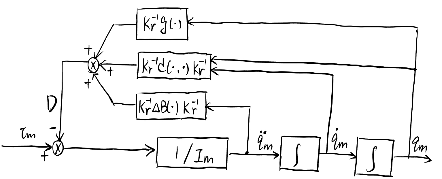
../_images/decentralized_control3.jpeg — Fig. 74 Dynamics diagram of a motor-driven robot arm.#

As shown in both (64) and Fig. 74, if we ignore the coupling term $\boldsymbol{D}$,

\[\boldsymbol{I}_m\boldsymbol{\ddot{q}}_m=\boldsymbol{\tau}_m,\]

This means that if we ignore complex term $\boldsymbol{D}$, each joint is a single-in-single-output system (because $\boldsymbol{I}_m$ is a diagonal matrix). However, the coupling term $\boldsymbol{D}$ in (64) prevents us from considering so. How do we overcome this in our control design?

Important

In our control design, we consider the each joint as a single-in-single-out system, but view the complex coupling effect term $\boldsymbol{D}$ as a disturbance input to each joint.

Minimal material on control basics

Please read my hand-writing note on control basics, in order to help you understand the following content of this chapter.

Minimal notes on control basics

Minimal Introduction to Closed-Loop (Feedback) Control Systems

A typical closed-loop control diagram is shown below. Here, $\theta_r$ is the reference input; $\theta_m$ is the output; $D$ is the disturbance; $G(s)$ is the transfer function of the plant to be controlled; $C(s)$ is the controller; $H(s)$ is the backward pass transfer function (usually a constant to model the sensor). The goal of control design is to find $C(s)$ such that $\theta_m$ is able to track $\theta_r$, while $D$ has as little effect on $\theta_m$ as possible.

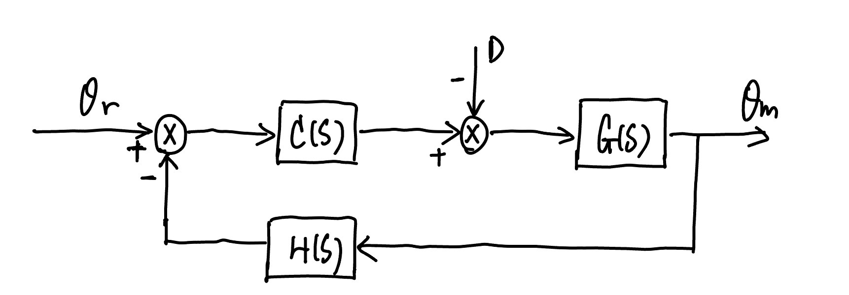
../_images/fd_control2.jpeg — Fig. 75 A typical control system diagram#

For the above control system, the forward path transfer function is

\[C(s)G(s)\]

The backward path transfer function is

\[H(s)\]

The open loop transfer function is

\[C(s)G(s)H(s)\]

The input-to-output transfer function is

\[ \frac{\Theta_m(s)}{\Theta_r(s)}=\frac{C(s)G(s)}{1+C(s)G(s)H(s)} \]

The disturbance-to-output transfer function is

\[ \frac{\Theta_m(s)}{D(s)}=\frac{G(s)}{1+C(s)G(s)H(s)} \]

The input ($\theta_r$) to output ($\theta_m$) response of the closed-loop system will be determined by the roots of the characteristics equation

\[1+C(s)G(s)H(s)=0\]

Single-Joint System Diagram#

In the reminder of this chapter, i will use ${\theta}_m$ and $q_m$ interchangeably as the variable of each joint, droping the subscript of joint index. For a single joint, the dynamics equation at that joint is a row of (64), writing as

(65)#\[ I_m\ddot{\theta}_m+D=\tau_m \]

Let’s recall the DC motor model in our previous chapter:

(66)#\[ \tau_m=k_ti_a=k_t\frac{(G_vv_c-k_v\dot{\theta}_m)}{R_a}=k_t\frac{(v_a-k_v\dot{\theta}_m)}{R_a} \]

where ${k}_{t}$ is the torque constants; ${i}_{a}$ is the armature current; ${v}_{a}$ is the vector of armature voltage; ${R}_{a}$ is the armature resistance; ${k}_{v}$ is the back EMF constant; $v_a=G_vv_c$ with $\boldsymbol{v}_{c}$ is the voltage input of the servomotor, and $G_v$ is voltage amplifier. Those parameters have been shown in previous chapter.

Equaling (65) and (66), one has

(67)#\[ I_m\ddot{\theta}_m+D=\tau_m=I_m\ddot{\theta}_m+\frac{k_t}{R_a}(\frac{DR_a}{k_t})=k_t\frac{(v_a-k_v\dot{\theta}_m)}{R_a} \]

The above (67) corresponds to the following diagram

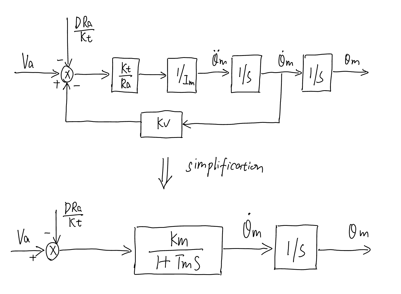
../_images/motor_model3.jpeg — Fig. 76 Diagram of a single motor-joint model, with coupled joint term $D$ treated as disturbance.#

For the above diagram, the input ($v_a$) to output ($\theta_m$) transfer function $G(s)$ is

(68)#\[ G(s)=\frac{{\Theta}(s)}{V_a(s)}=\frac{k_m}{s(1+T_ms)}\]

with

\[ k_m=\frac{1}{k_v} \qquad\qquad T_m=\frac{R_aI_m}{k_tk_v} % \frac{\frac{k_t}{R_aI_ms}}{1+\frac{k_t}{R_aI_ms}k_v}= \]

The input ($v_a$) to output velocity ($\dot{\theta}_m$) transfer function is

\[\frac{\dot{\Theta}(s)}{V_a(s)}=\frac{k_m}{1+T_ms}\]

The single joint system in Fig. 76 is the plant $G(s)$ we want to design the controller $C(s)$ for.

Position Feedback Control Design#

The transfer function $G(s)$ for the single joint system (Fig. 76) is in (68), rewritten below

\[G(s)=\frac{k_m}{s(1+T_ms)}\]

We want to design a proportional-integral controller

\[\begin{gathered} C_{P}(s)=K_{P} \frac{1+s T_{P}}{s} \end{gathered}\]

with $K_P$ and $T_P$ are controller parameters.

The control diagram for the single joint system (Fig. 76) is shown below (note that the backward pass constant $k_{TP}$ is given and a constant, which can be thought of as the sensor gain).

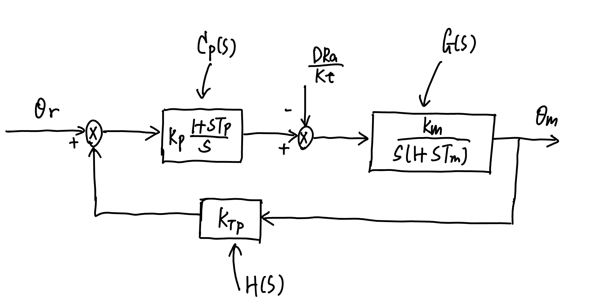
../_images/p_control2.jpg — Fig. 77 Control diagram of single-joint system#

On the diagram Fig. 77, the transfer function of the forward path is

\[G(s)C_P(s)=\frac{k_{m} K_{P}\left(1+s T_{P}\right)}{s^{2}\left(1+s T_{m}\right)}\]

The transfer function of the backward pass is

\[H(s)=k_{T P}\]

The open loop transfer function is

\[ G(s)C_P(s)H(s)=\frac{k_{T P}k_{m} K_{P}\left(1+s T_{P}\right)}{s^{2}\left(1+s T_{m}\right)} \]

The closed-loop input-to-output transfer function is

(69)#\[\frac{\Theta_{m}(s)}{\Theta_{r}(s)}=\frac{C_P(s)G(s)}{1+C_P(s)G(s)H(s)}=\frac{{k_{m}K_P(1+T_Ps)}}{k_{TP}k_{m}K_P(1+T_Ps)+s^2(1+sT_m)},\]

Input-to-output stability analysis#

To analyze the input-to-output stability of the closed-loop control system (69), we look at the roots (also called poles) of its characteristic equation, which can be factorized into the following form

(70)#\[{k_{TP}k_{m}K_P(1+T_Ps)+s^2(1+sT_m)} = {\left({\omega_{n}^{2}}+{2 \zeta }{\omega_{n}}s+{s^{2}}\right)(1+s \tau)}=0\]

The roots (also called poles) to the characteristics equation (70) is

\[\begin{split} \begin{aligned} s_1&=-\zeta \omega_{n}, + j \sqrt{1-\zeta^{2}} \omega_{n}\\ s_2&=-\zeta \omega_{n}, - j \sqrt{1-\zeta^{2}} \omega_{n}\\ s_3&=-1 / \tau \end{aligned} \end{split}\]

Here, $\omega_{n}$ and $\zeta$ are the natural frequency and damping ratio for the complex roots $s_1$ and $s_2$, and $s_3$ is a real pole. Please see my Minimal notes on control basics for explaination of how the values of $\omega_{n}$, $\zeta$ and $s_3$ effect the time-domain performance of the closed-loop control system.

The location of the above poles $(s_1, s_2, s_3)$ on s-plane depends on the of the open-loop gain

(71)#\[\frac{k_{m} K_{P} k_{T P} T_{P}}{T_{m}}\]

The root locus (i.e., the trajectory of the above poles on $s-$plane) can be drawn by taking different open loop gain value (71). Here, we derive into two cases:

If $T_{P}<T_{m}$, the root locus is shown. Because there is always a pole (root) living on the right-half s-plane regardless of the choice of $\frac{k_{m} K_{P} k_{T P} T_{P}}{T_{m}}$, the closed-loop control system (69) thus is inherently unstable.

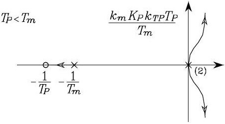
Fig. 78 Root locus when $T_{P}<T_{m}$#
If $T_{P}>T_{m}$, the root locus is shown as below. First, all poles can be located on the left half of s-plane, thus closed-loop control system (69) is stable. Also, as $T_{P}$ increases, the absolute value of the real part of the two complex poles, ($s_1$ and $s_2$) tending towards the asymptotes increases too, and the system has faster time response (please see my Minimal notes on control basics for explaination)

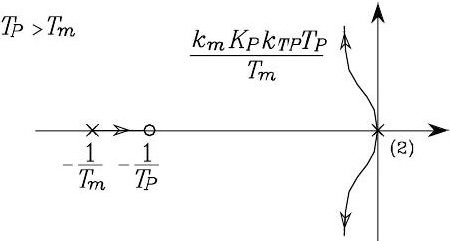
Fig. 79 Root locus when $T_{P}>T_{m}$#

Disturbance-to-output performance#

Final value theorem

If a continuous signal $f(t)$ has its Laplace transformation $F(s)$, then the final value theorem states

\[\lim_{t\rightarrow\infty}f(t)=\lim_{s\rightarrow 0}sF(s)\]

The closed-loop disturbance-to-output transfer function is

\[\frac{\Theta_{m}(s)}{D(s)}=-\frac{\frac{R_a}{K_t}G(s)}{1+C(s)G(s)H(s)}=-\frac{\frac{R_a}{K_t}k_ms}{k_{TP}k_{m}K_P(1+T_Ps)+s^2(1+sT_m)}\]

If $\theta_r(t)=0$ (i.e., no input signal), based on the final value thoerem (see the above), we have

\[\lim_{t\rightarrow \infty} {\theta_{m}(t)}= \lim_{s\rightarrow 0} s{\Theta_{m}(s)}=\lim_{s\rightarrow 0} s\frac{\Theta_{m}(s)}{D(s)}{D(s)}\]

thus,

\[\begin{split}\lim_{t\rightarrow \infty} {\theta_{m}(t)}= \begin{cases} 0\qquad &\text{if}\quad D(t)\,\,\text{is constant signal}\\ \frac{R_a}{K_t}\frac{1}{K_{P} k_{T P}} \qquad &\text{if}\quad D(t)\,\,\text{is ramp signal, such as $D(t)=vt$ }\\ \end{cases}\end{split}\]

Hence, the controller can mitigate the effect of disturbance, and the mitigation is controlled by

\[K_{P} k_{T P}\]

which can be interpreted as the disturbance rejection factor for velocity (or higher-order) disturbance. Increasing $K_{P}$ can help with reducing the effect of $D$, but too high $K_P$ can lead to unacceptable oscillations of the output, as implied from the root locus.