Motion Planning#
Motion planning is the problem of finding a robot motion from start state to a goal state that avoids obstacles in the environment (also statisfies other constraints).
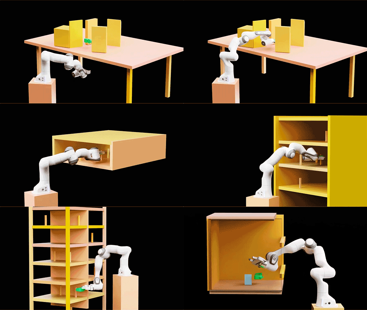
Fig. 41 Robot arm motion planning#
Configuration Space#
Configuration of a robot: a representation of a robot pose, typically using the joint vector \(q\in R^n\).
Configuration space (C-Space): the space that contains all possible robot configurations.
Free space \(C_{free}\): the subset of configurations where the robot does not contact any obstacle.
Obstacle space \(C_{obs}\): the subset of configurations where the robot is in collision with an obstacle.
The robot configuration space \(C\) is a union of free space \(C_{free}\) and obstacle space \(C_{obs}\):
State of a robot: is defined as \(x=(q,v)\), joining the robot configuration \(q\) and its velocity \(v=\dot{q}\)
Equation of motion (dynamics) of a robot: an ordinary differentiable equation (ODE) defined on the robot state \(x\) and control input \(u\) (e.g., the input force).
Some examples:
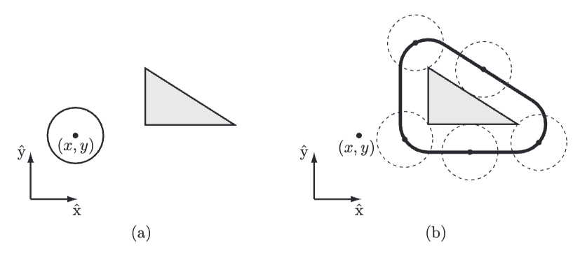
Fig. 42 (a) A circular mobile robot (open circle) and a workspace obstacle (gray triangle). The configuration of the robot is represented by \((x, y)\) at its center. (b) In C-space, the obstacle is “grown” by the radius of the robot and the robot is treated as a point. Any \((x, y)\) configuration outside the bold line is collision-free.#
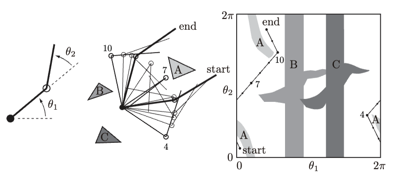
Fig. 43 (Left) The joint angles of a 2R robot arm. (Middle) The arm navigating among obstacles A, B, and C. (Right) The same motion in C-space. Three intermediate points, 4, 7, and 10, along the path are labeled.#
Optimization-based motion planning (NOT convered)#
Robot motion is generated by solving an optimization problem that minimizes (or maximizes) a given cost function (such as minimal jerk, control energy) while satisfying various constraints, such as obstacle avoidance and robot dynamics. Mathmatically,
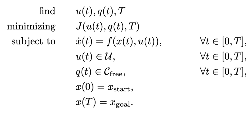
Fig. 44 General formulation for optimization-based robot motion planning#
Some methods (Please read the original paper if you are interested):
Sampling-based motion planning (focused here)#
Probabilistic Roadmap (PRM)#
Python example code (copyright, authored by IRIS Lab): https://colab.research.google.com/drive/1TvEIeUeZnZjJOjU33IVWLnP43DrFXxVY?usp=sharing
The basic PRM algorithm in robot configuration space Fig. 45 is as follows:
Step 1: Sample \(N\) configurations at random from the C-space, as shown in Fig. 46. Check all sampled configurations and remove those in the obstacle sapce. Only add the samples in free space and start and goal to the roadmap (also known as milestones), as shown in Fig. 47.
Step 2: Each milestone is linked by straight paths to its nearest neighbors. The collision-free links are retained as local paths to form the PRM, as shown in Fig. 48.
Step 3: Search for a path from the start to the goal using A* search or Dijkstra’s search algorithms, as shown in Fig. 49.
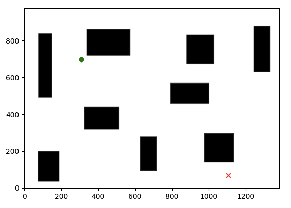
Fig. 45 Configuration space: balck blocks show obstacle space and the while show free space. The start is shown in green and goal in red.#
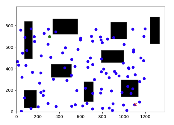
Fig. 46 Sample \(N\) configurations at random from the C-space.#
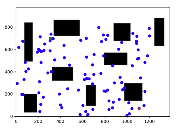
Fig. 47 Only add the samples in free space and the start and goal to the roadmap (also known as milestones).#
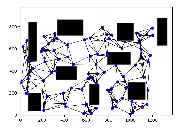
Fig. 48 Each milestone is linked by straight paths to its nearest neighbors. The collision-free links are retained as local paths to form the PRM#
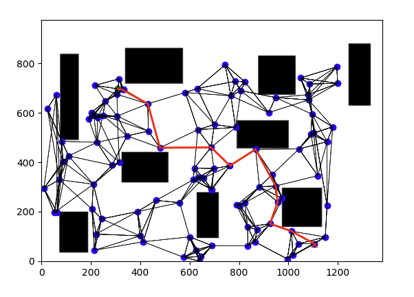
Fig. 49 Search for a path from the start to the goal using A* search algorithms.#
Rapidly-exploring Random Trees (RRTs)#
Python example code (copyright, authored by IRIS Lab): https://colab.research.google.com/drive/1fxMlKzIWIWr6Qq49wTmTsIAJz5pp0ing?usp=sharing
The basic RRT algorithm is as follows (from https://arxiv.org/pdf/1105.1186)
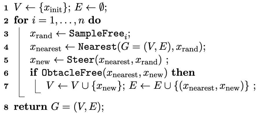
Fig. 50 Basic RRT algorithm#
A visualization of how RRT works step by step in 2D space is shown as follows.
CREDIT: all the figures are taken from rey’s blog (https://rrwiyatn.github.io/blog/robotik/2020/05/16/rrt.html)
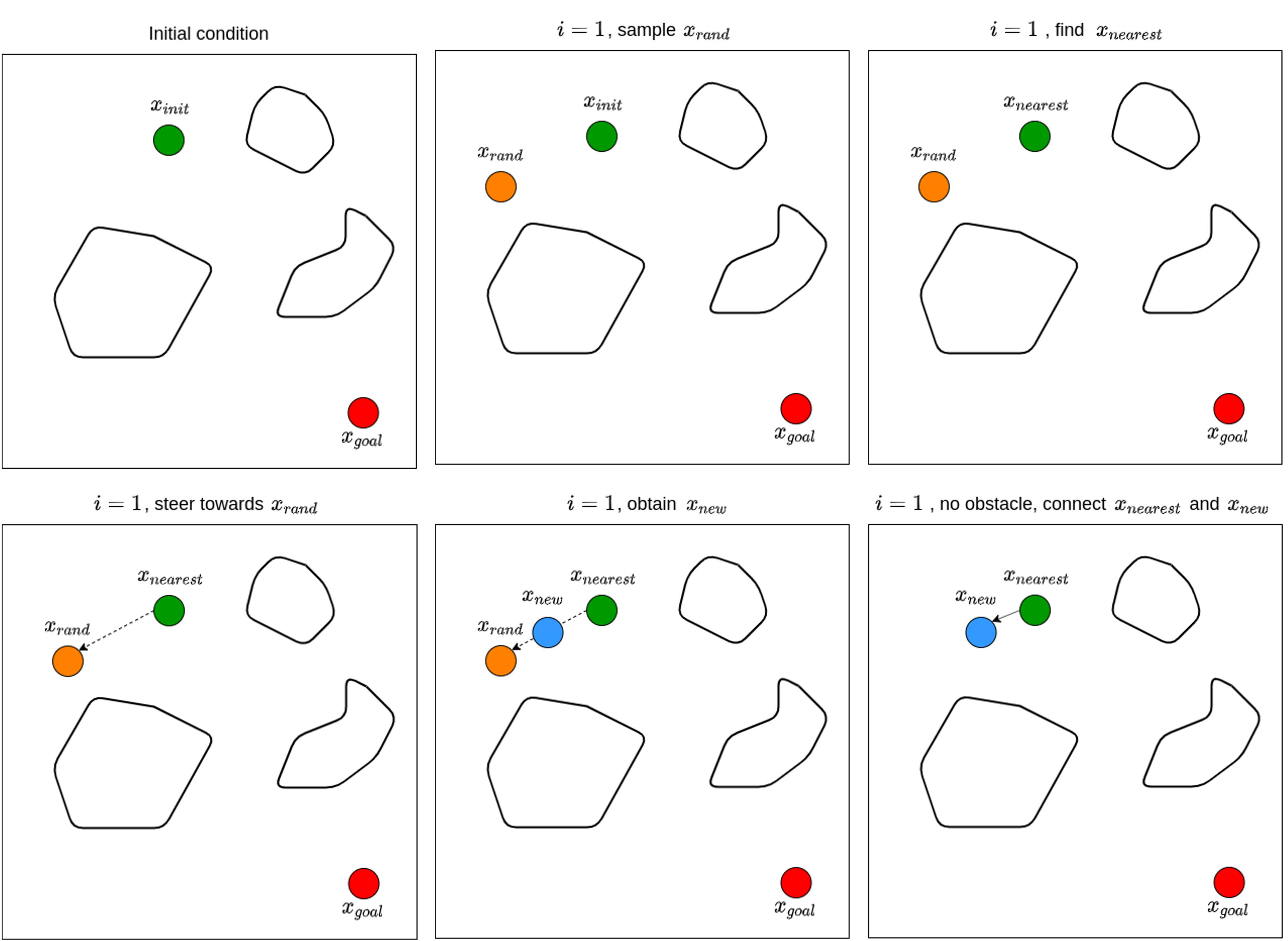
Fig. 51 The 1st iteration in RRT algoritm#
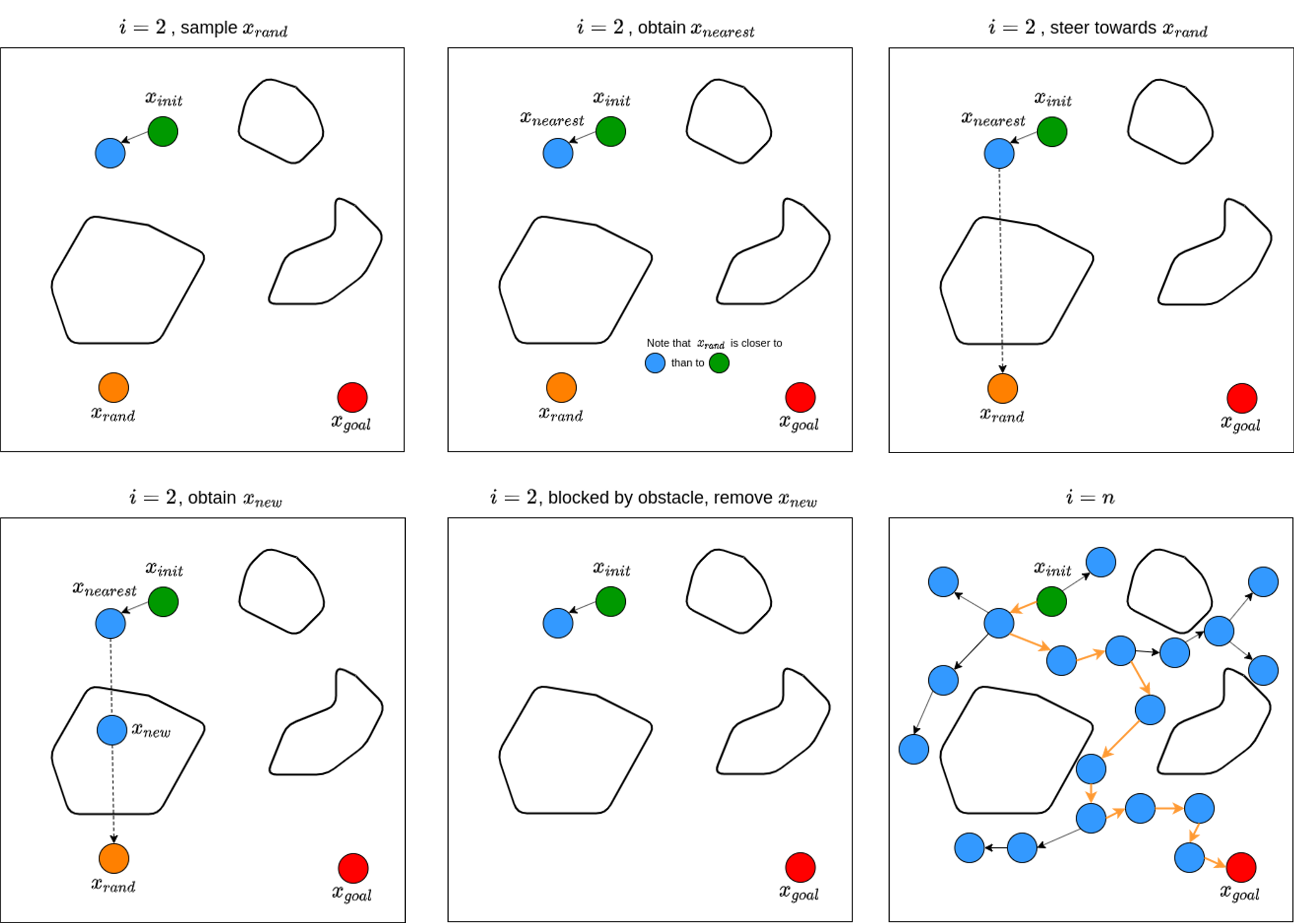
Fig. 52 The 2nd iteration of RRT to n-th iteration#
Variants of RRT#
bidirectional or multi-directional RRT
RRT*: Swap new point in as parent for nearby vertices who can be reached along shorter path through new point than through their original (current) parent.
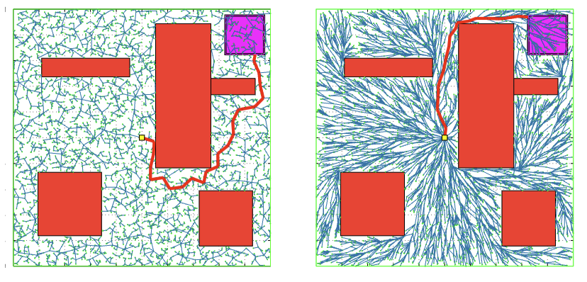
Fig. 53 (Left) The tree generated by an RRT after 5,000 nodes. The goal region is the square at the top right corner, and the shortest path is indicated. (Right) The tree generated by RRT* after 5,000 nodes. Figure from original paper (https://arxiv.org/abs/1105.1186).#
Smoothing#
Randomized motion planners tend to find not so great paths for execution: very jagged, often dynamially infeasbile. So, people usually do smoothing before using the planned path.
Subdividing and Reconnecting: A local planner can be used to attempt a connection between two distant points on a path. If this new connection is collision free, it replaces the original path segment. Since the local planner is designed to produce short, smooth, paths, the new path is likely to be shorter and smoother than the original. This test-and-replace procedure can be applied iteratively to randomly chosen points on the path. Another possibility is to use a recursive procedure that subdivides the path first into two pieces and attempts to replace each piece with a shorter path; then, if either portion cannot be replaced by a shorter path, it subdivides again; and so on.
Nonlinear Optimization: With the obtained path as initial condition, one can define an objective function that includes smoothness in state, control, small control inputs, etc, and optimize such objective function for smoother path.
