Robot Configuration

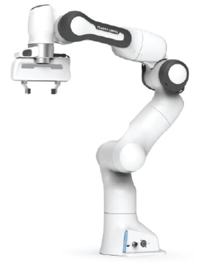
Fig. 1 Franka research robot arm

A robot manipulator is mechanically constructed by

• a set of rigid bodies, each body called a link,

• joints, connecting two consecutive links and providing motion constraints (degrees of freedom)

  

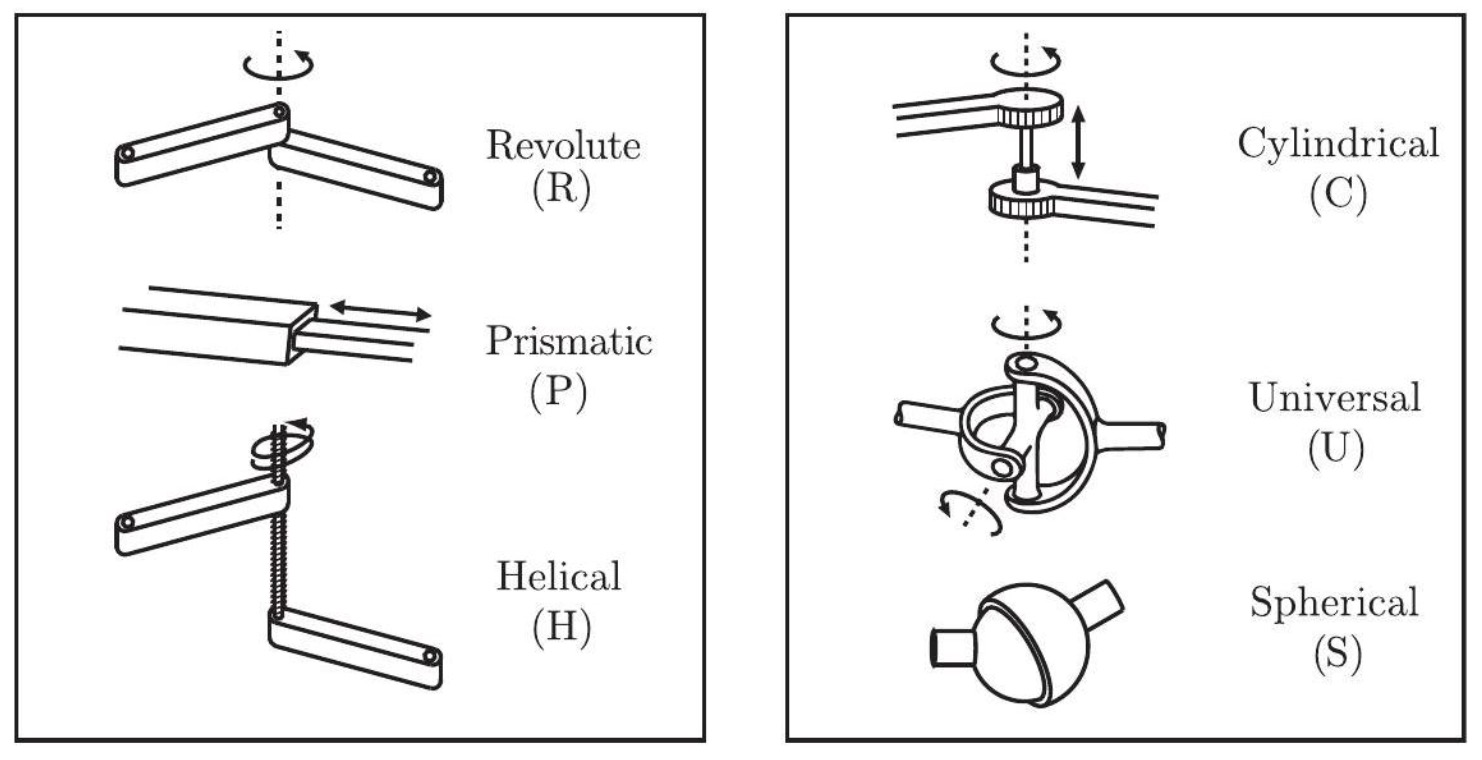
  Fig. 2 Different type of joints

• actuators, such as electric/hydraulic/pneumatic actuators, deliver forces or torques that cause the robot’s links to move,

  

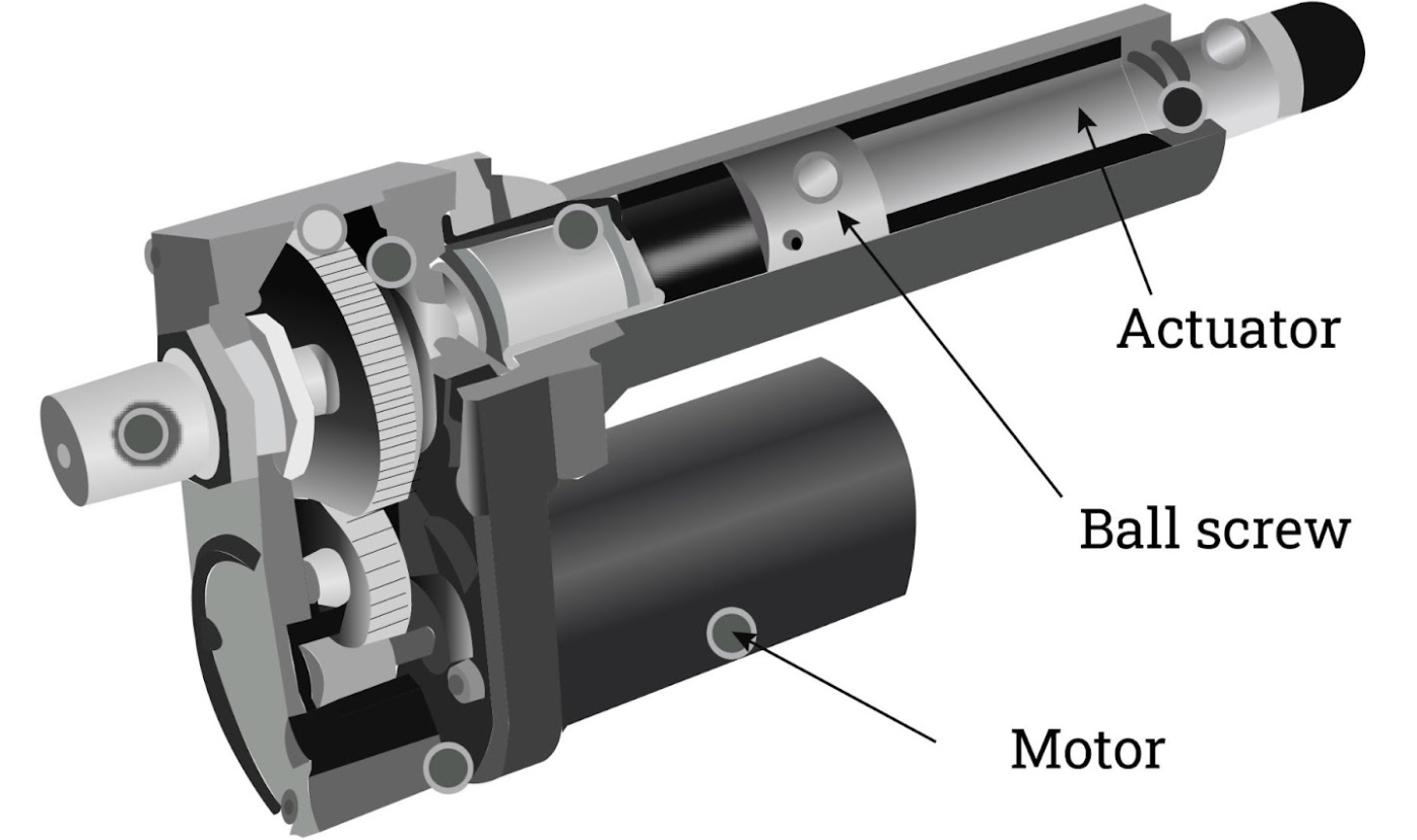
  Fig. 3 Electric actuators

  

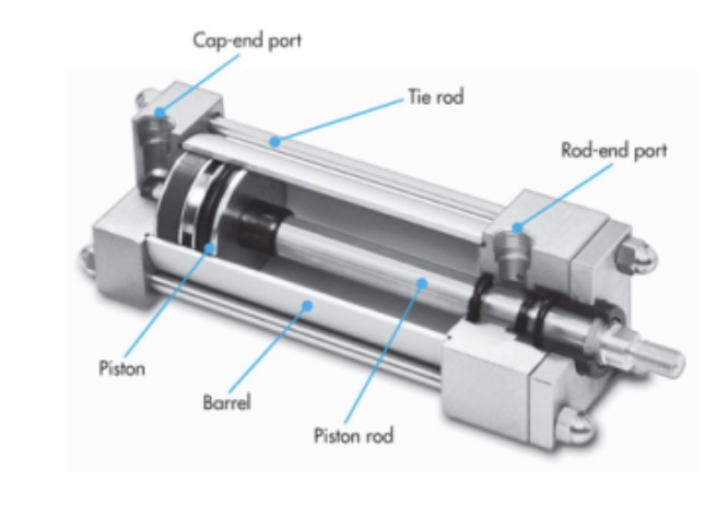
  Fig. 4 Hydralic actuator

• an end effector, such as a gripper or hand, is attached to a specific link for specific tasks.

  

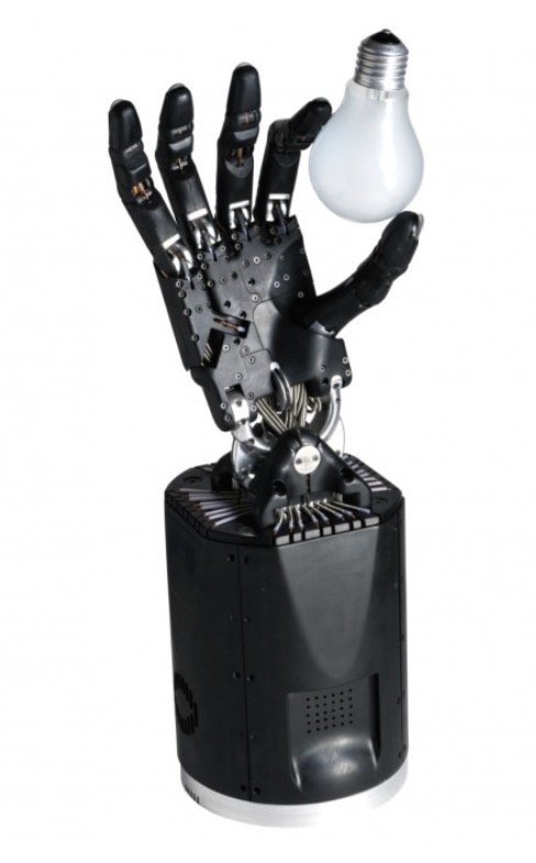
  Fig. 5 The Shadow Hand

The typical structure of a robot arm is an open kinematic chain. From a topological viewpoint, a kinematic chain is open when there is only one sequence of links connecting the two ends of the chain. Alternatively, kinematic chain is closed when a sequence of links forms a loop. This course mainly focuses on open chain arms.

MuJoCo Simulator Introduction

MuJoCo (Multi-Joint dynamics with Contact) is a physics engine designed for the simulation and control of robots and other articulated mechanisms. It is widely used in robotics research for its speed, accuracy, and support for advanced features such as soft contacts and complex constraints.

Key Features:

• Fast and accurate simulation of rigid body dynamics

• Support for soft and hard contacts

• Flexible model specification using XML

• Widely used in reinforcement learning and robotics research

Getting Started:

To use MuJoCo, you need to:

1. Install MuJoCo (UI) from google-deepmind/mujoco

2. Download Example Model:** franka_fr3.zip

3. Unzip and drag it into UI to simulate the Franka Research 3 Robot arm.

Configuration

Important

The configuration of a robot is a complete specification of the position of every point of the robot. Since a robot’s links are rigid and of a known shape, only a few coordinates are needed to represent its configuration.

For example, in the following figure, the configuration of a door can be represented by the hinge angle \(\theta\). The configuration of a point on a plane can be represented by two coordinates, \((x, y)\). The configuration of a coin lying heads up on a flat table can be represented by three coordinates: \((x, y)\) that specifies the location of a particular point on the coin, and \((\theta)\) that specifies the coin’s orientation.

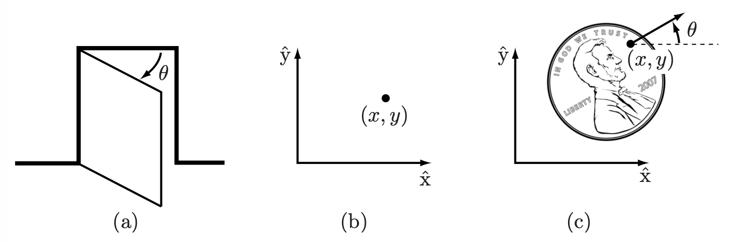
Fig. 6 (a) The configuration of a door is represented by the angle \(\theta\). (b) The configuration of a point in a plane is represented by coordinates \((x, y)\). (c) The configuration of a coin (heads up) on a table is represented by \((x, y, \theta)\).

Degrees of Freedom

Important

The minimum number \(n\) of coordinates needed to represent the configuration of a robot is the degree of freedom (dof). The \(n\)-dimensional space containing all possible configurations/coordinates of a robot is called the configuration space (C-space). A configuration of a robot is represented by a point in its C-space.

General Rule

We have the following general rule to determine the number of dof of a robot:

Important

degrees of freedom = number of variables - number of independent constraints

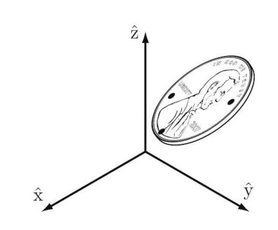
Fig. 7 A coin in 3D space

Example: consider a coin in 3D space in Fig. 7, the coordinates for the three points \(A, B\), and \(C\) are given by \(\left(x_{A}, y_{A}, z_{A}\right),\left(x_{B}, y_{B}, z_{B}\right)\), and \(\left(x_{C}, y_{C}, z_{C}\right)\), respectively. Each point has 3 dof, and therefore total dof are 9. However, consider the rigid body assumption, meaning that distance between any two points are fixed. This introduces 3 constraints. Therefore, a rigid body moving in 3D space has 9-3=6 dof.

• A rigid body moving in 3-dimensional space has \(m=6\) dof.

• A rigid body moving in a 2-dimensional plane has \(m=3\) dof.

DOF of Different Joint Types

In a robot, a joint can be viewed as providing freedoms to allow one rigid body to move relative to another. It can also be viewed as providing constraints on the possible motions of the two rigid bodies it connects. The following table summarizes the freedoms and constraints provided by the various joint types.

Joint type	dof (f)	# of constraints between two bodies in 3D space (c)
Revolute (R)	1	5
Prismatic (P)	1	5
Helical (H)	1	5
Cylindrical (C)	2	4
Universal (U)	2	4
Spherical (S)	3	3

Let \(f\) be the number of freedoms provided by joint \(i\), and \(c\) be the number of constraints provided by joint \(i\), where \(f+c=m\). \(m=3\) for planar mechanisms and \(m=6\) for 3D mechanisms.

Grübler’s Formula

Important

Consider a mechanism consisting of \(L\) links, where the ground is also regarded as a link. Let \(J\) be the number of joints, \(m\) be dof of a rigid body (\(m=3\) for planar mechanisms and \(m=6\) for 3D mechanisms), \(f_{i}\) be the number of freedoms provided by joint \(i\), and \(c_{i}\) be the number of constraints provided by joint \(i\), where \(f_{i}+c_{i}=m\) for all \(i\). Then the Grübler’s formula for dof of the mechanism is

\[\begin{split} \begin{aligned} \operatorname{dof} & =\underbrace{m(L-1)}_{\text {total number of freedoms for all rigid bodies }}-\underbrace{\sum_{i=1}^{J} c_{i}}_{\text {joint constraints }} \\ & =m(L-1)-\sum_{i=1}^{J}\left(m-f_{i}\right) \\ & =m(L-1-J)+\sum_{i=1}^{J} f_{i} . \end{aligned} \end{split}\]

This formula holds only if all joint constraints are independent. If they are not independent then the formula provides a lower bound on the number of degrees of freedom.

Below are some examples of using Grubler’s Formula to find the DoFs of different machenisms.

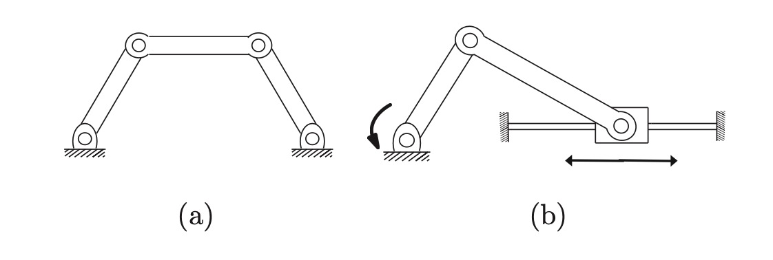
Fig. 8 (a) Four-bar linkage and (b) Slider-crank mechanism.

(Four-bar linkage): \(L=4, J=4\), and \(f_{i}=1, i=1, \ldots, 4\). Thus, \(\operatorname{dof}\)=1.
Slider-crank: \(L=4\), \(J=4,\) and \(f_{i}=1, i=1, \ldots, 4\). Thus, \(\operatorname{dof}\)=1.

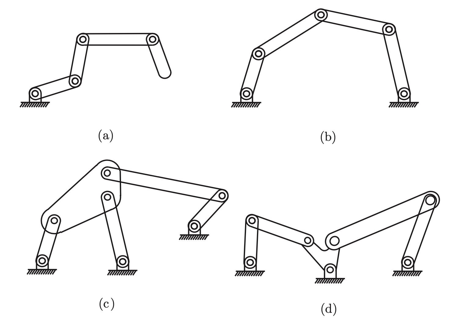
Fig. 9 (a) \(k\)-link planar serial chain. (b) Five-bar planar linkage. (c) Stephenson six-bar linkage. (d) Watt six-bar linkage.

The \(k\)-link planar robot: \(L=k+1\), \(J=k\), \(f_{i}=1\) for all \(i\). Thus, \(\operatorname{dof}=3*((k+1)-1-k)+k=k\).
The five-bar linkage: \(L=5\), \(J=5\), each \(f_{i}=1\). Therefore, \(\operatorname{dof}=3*(5-1-5)+5=2\).
Stephenson six-bar linkage: \(L=6, J=7\), and \(f_{i}=1\) for all \(i\). Therefore, \(\operatorname{dof}=3*(6-1-7)+7=1\).
Watt six-bar linkage: \(L=6, J=7\), and \(f_{i}=1\) for all \(i\). Therefore, \(\operatorname{dof}=3*(6-1-7)+7=1\).

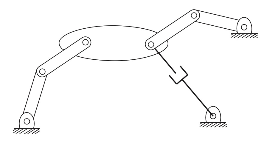
Fig. 10 A planar mechanism with two overlapping joints.

The planar mechanism in Fig. 10 has three links that meet at a single point on the right of the large link. Recalling that a joint by definition connects exactly two links, the joint at this point should not be regarded as a single revolute joint. Rather, it should be counted as two revolute joints overlapping each other. The mechanism consists of eight links \((L=8)\), 8 revolute joints, and 1 prismatic joint. The Grübler’s formula:

\[\operatorname{dof}=3*(8-1-9)+9*(1)=3\]

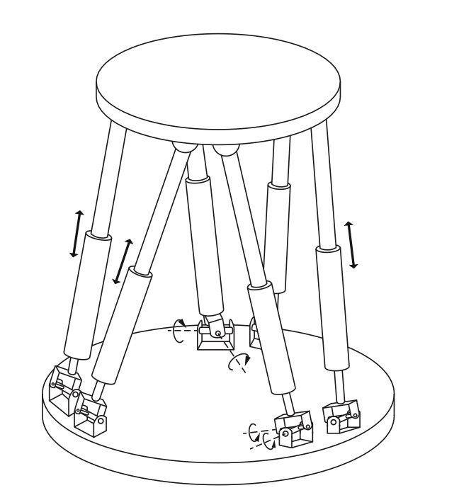
Fig. 11 Stewart-Gough platform

The Stewart-Gough platform consists of two platforms - the lower one is regarded as ground, the upper one mobile - connected by six universal-prismatic-spherical (UPS) legs. The total number of links is \(14(L=14)\). There are six universal joints (for each, \(f_{i}=2\) ), six prismatic joints (for each, \(f_{i}=1\) ), and six spherical joints (for each, \(f_{i}=3\) ). The total number of joints is 18 . Using Grübler’s formula, we have

\[\operatorname{dof}=6*(14-1-18)+6*(1)+6*(2)+6*(3)=6 .\]

Workspace of Robot Arms

The workspace is the space of the environment a robot arm’s end-effector can access. Its shape and volume depend on the robot arm’s structure as well as mechanical joint limits. The workspace is independent of the task. In the following, below is the workspace of different commonly used robot arms.

Cartesian robot arm includes three prismatic joints whose axes typically are mutually orthogonal.

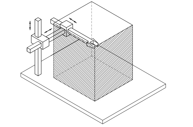
Fig. 12 Cartesian robot arm and its workspace

Cylindrical robot arm differs from Cartesian in that the first prismatic joint is replaced with a revolute joint.

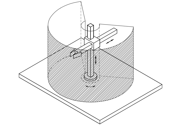
Fig. 13 Cylindrical robot arm and its workspace

Spherical robot arm differs from cylindrical in that the 2nd prismatic joint is replaced with a revolute joint.

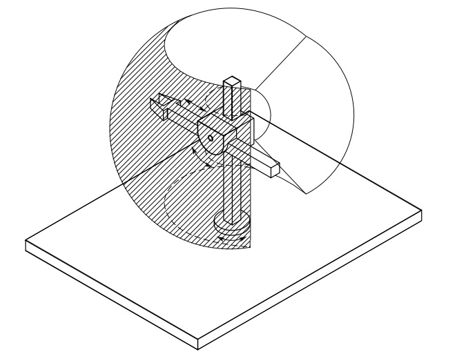
Fig. 14 Spherical robot arm and its workspace

A special robot arm is SCARA robot arm, which has the feature that all the axes of motion are parallel.

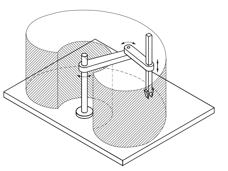
Fig. 15 SCARA robot arm and its workspace

Anthropomorphic robot arm has three revolute joints; the revolute axis of the first joint is orthogonal to the axes of the other two which are parallel.

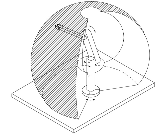
Fig. 16 Anthropomorphic robot arm and its workspace