Basic Kinematics

The pose of a rigid body in 3D space is described by its position and orientation with respect to a reference frame. As in Fig. 17, let \(O-xyz\) be the reference frame and \(\{\boldsymbol{x}, \boldsymbol{y}, \boldsymbol{z}\}\) be the unit vectors of the frame axes. To represent the pose of the rigid body, we pick a fixed point \(O^\prime\) on the rigid body, and attach an body frame \(O^{\prime}-x^{\prime} y^{\prime} z^{\prime}\) to the body, with origin \(O^{\prime}\) and \(\{\boldsymbol{x}^{\prime}, \boldsymbol{y}^{\prime}, \boldsymbol{z}^{\prime}\}\) being the unit vectors.

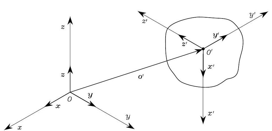
Fig. 17 Pose of a rigid body in a reference frame

The position of the rigid body is defined as a position vector \(\boldsymbol{o}^{\prime}\) pointing from the reference frame origin \(O\) to the body frame origin \(O'\). We express \(\boldsymbol{o}^{\prime}\) in terms of \(\{\boldsymbol{x}, \boldsymbol{y}, \boldsymbol{z}\}\) of reference frame:

\[\begin{split} \boldsymbol{o}^{\prime}=o_{x}^{\prime} \boldsymbol{x}+o_{y}^{\prime} \boldsymbol{y}+o_{z}^{\prime} \boldsymbol{z} :=\left[\begin{array}{c} o_{x}^{\prime} \\ o_{y}^{\prime} \\ o_{z}^{\prime} \end{array}\right] =\left[\begin{array}{c} {\boldsymbol{o}^{\prime}}^T \boldsymbol{x} \\ {\boldsymbol{o}^{\prime}}^T \boldsymbol{y} \\ {\boldsymbol{o}^{\prime}}^T \boldsymbol{z} \end{array}\right] \end{split}\]

where \(o_{x}^{\prime}, o_{y}^{\prime}, o_{z}^{\prime}\) are called the coordinates of vector \(\boldsymbol{o}^{\prime}\) and are the projections of \(\boldsymbol{o}^{\prime}\) in \(\{\boldsymbol{x}, \boldsymbol{y}, \boldsymbol{z}\}\).

To describe the orientation of the rigid body, we find the coordinates of each unit axis \(\{\boldsymbol{x}^{\prime}, \boldsymbol{y}^{\prime}, \boldsymbol{z}^{\prime}\}\) in the reference frame:

\[\begin{split} \begin{aligned} & \boldsymbol{x}^{\prime}=x_{x}^{\prime} \boldsymbol{x}+x_{y}^{\prime} \boldsymbol{y}+x_{z}^{\prime} \boldsymbol{z} \\ & \boldsymbol{y}^{\prime}=y_{x}^{\prime} \boldsymbol{x}+y_{y}^{\prime} \boldsymbol{y}+y_{z}^{\prime} \boldsymbol{z} \\ & \boldsymbol{z}^{\prime}=z_{x}^{\prime} \boldsymbol{x}+z_{y}^{\prime} \boldsymbol{y}+z_{z}^{\prime} \boldsymbol{z} \end{aligned} \end{split}\]

Rotation Matrix and its Properties

We write the above into the following matrix notation:

(1)\[\begin{split} \boldsymbol{R}=\left[\begin{array}{lll} \boldsymbol{x}^{\prime} & \boldsymbol{y}^{\prime} & \boldsymbol{z}^{\prime} \end{array}\right]=\left[\begin{array}{ccc} x_{x}^{\prime} & y_{x}^{\prime} & z_{x}^{\prime} \\ x_{y}^{\prime} & y_{y}^{\prime} & z_{y}^{\prime} \\ x_{z}^{\prime} & y_{z}^{\prime} & z_{z}^{\prime} \end{array}\right]=\left[\begin{array}{lll} \boldsymbol{x}^{\prime T} \boldsymbol{x} & \boldsymbol{y}^{\prime T} \boldsymbol{x} & \boldsymbol{z}^{\prime T} \boldsymbol{x} \\ \boldsymbol{x}^{\prime T} \boldsymbol{y} & \boldsymbol{y}^{\prime T} \boldsymbol{y} & \boldsymbol{z}^{\prime T} \boldsymbol{y} \\ \boldsymbol{x}^{\prime T} \boldsymbol{z} & \boldsymbol{y}^{\prime T} \boldsymbol{z} & \boldsymbol{z}^{\prime T} \boldsymbol{z} \end{array}\right]\end{split}\]

with each column being the coordinates/projections of each unit vector \(\{\boldsymbol{x}^{\prime}, \boldsymbol{y}^{\prime}, \boldsymbol{z}^{\prime}\}\) in \(\{\boldsymbol{x}, \boldsymbol{y}, \boldsymbol{z}\}\). \(\boldsymbol{R}\) is called rotation matrix.

Some properties of Rotation Matrix:

• Mutual orthogonality: \(\boldsymbol{x}^{\prime T} \boldsymbol{y}^{\prime}=0\), \(\boldsymbol{y}^{\prime T} \boldsymbol{z}^{\prime}=0\), and \(\boldsymbol{z}^{\prime T} \boldsymbol{x}^{\prime}=0\)

• Unity: \(\boldsymbol{x}^{\prime T} \boldsymbol{x}^{\prime}=1\), \(\boldsymbol{y}^{\prime T} \boldsymbol{y}^{\prime}=1\), and \(\boldsymbol{z}^{\prime T} \boldsymbol{z}^{\prime}=1\)

• Orthogonal matrix: \(\boldsymbol{R}^{T} \boldsymbol{R}=\boldsymbol{I}_{3} \quad \rightarrow \quad \boldsymbol{R}^{T}=\boldsymbol{R}^{-1}\)

• The determinant (righ-hand rule convention): \(|\det \boldsymbol{R}|=1\)

Elementary Rotations

Consider the origin of the body frame coincides with the origin of the reference frame. The orientation of a body frame can be obtained by the rotating the reference frame about its axes. Below, we consider right-handed rotation convention: rotations are positive if counter-clockwise about a axis.

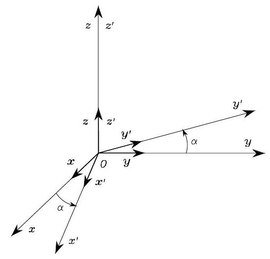
Fig. 18 Rotation of frame \(O- x y z\) by an angle \(\alpha\) about axis \(\boldsymbol{z}\)

As shown in Fig. 18, suppose the body frame \(O- x^{\prime} y^{\prime} z^{\prime}\) is a result of rotating a reference frame \(O- x y z\) by an angle \(\alpha\) about the axis \(\boldsymbol{z}\). Then, the rotation matrix of \(O- x^{\prime} y^{\prime} z^{\prime}\) is

\[\begin{split} \boldsymbol{R}_{z}(\alpha)=\left[\begin{array}{ccc} \cos \alpha & -\sin \alpha & 0 \\ \sin \alpha & \cos \alpha & 0 \\ 0 & 0 & 1 \end{array}\right] \end{split}\]

Similarly, the rotation matrix for an angle \(\beta\) about axis \(\boldsymbol{y}\) is

\[\begin{split} \boldsymbol{R}_{y}(\beta) =\left[\begin{array}{ccc} \cos \beta & 0 & \sin \beta \\ 0 & 1 & 0 \\ -\sin \beta & 0 & \cos \beta \end{array}\right] \end{split}\]

and the rotation matrix for an angle \(\gamma\) about axis \(\boldsymbol{x}\) is

\[\begin{split} \boldsymbol{R}_{x}(\gamma) =\left[\begin{array}{ccc} 1 & 0 & 0 \\ 0 & \cos \gamma & -\sin \gamma \\ 0 & \sin \gamma & \cos \gamma \end{array}\right] . \end{split}\]

Transformation via Rotation Matrix

Passive Rotation

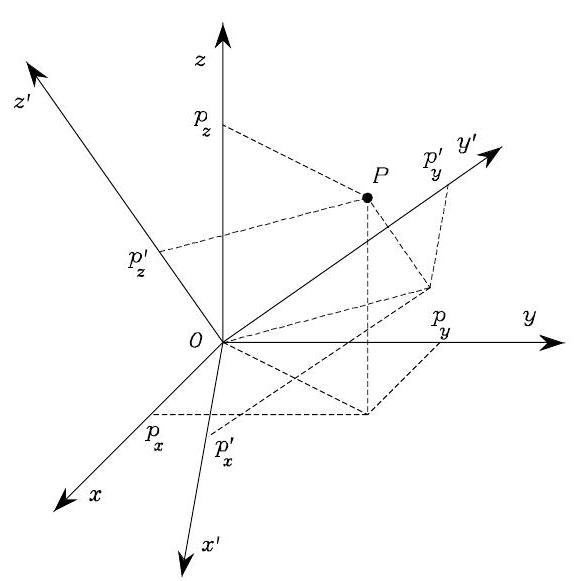
Fig. 19 Representation of a point \(P\) in two different coordinate frames

As in Fig. 19, consider that the origin of the body frame coincides with the origin of the reference frame, and that a point \(P\) expressed in \(O- x y z\) is

\[\begin{split} \boldsymbol{p}=p_{x} \boldsymbol{x} + p_{y} \boldsymbol{y} + p_{z}\boldsymbol{z} =\left[\begin{array}{c} p_{x} \\ p_{y} \\ p_{z} \end{array}\right] \end{split}\]

The same point can also be expressed in \(O- x^{\prime} y^{\prime} z^{\prime}\) as

\[\begin{split} \boldsymbol{p}=p_{x}^{\prime} \boldsymbol{x}^{\prime} + p_{y}^{\prime} \boldsymbol{y}^{\prime} + p_{z}^{\prime}\boldsymbol{z}^{\prime} = \left[\begin{array}{lll} \boldsymbol{x}^{\prime} & \boldsymbol{y}^{\prime} & \boldsymbol{z}^{\prime} \end{array}\right] \left[\begin{array}{c} p_{x}^{\prime} \\ p_{y}^{\prime} \\ p_{z}^{\prime} \end{array}\right]= \boldsymbol{R}\left[\begin{array}{c} p_{x}^{\prime} \\ p_{y}^{\prime} \\ p_{z}^{\prime} \end{array}\right] \end{split}\]

where we have applied the definition of the rotation matrix in (1). Therefore, one has

\[\begin{split} \left[\begin{array}{c} p_{x} \\ p_{y} \\ p_{z} \end{array}\right]=\boldsymbol{R}\left[\begin{array}{c} p_{x}^{\prime} \\ p_{y}^{\prime} \\ p_{z}^{\prime} \end{array}\right] \end{split}\]

and we simply write the above as

(2)\[ \boldsymbol{p}=\boldsymbol{R}\boldsymbol{p}^{\prime} \]

Passive rotation

\(\boldsymbol{R}\) is a transformation (mapping) for the coordinates of the same vector, from frame \(O- x^{\prime} y^{\prime} z^{\prime}\) to the to frame \(O- x y z\).

Active Rotation

In another perspective to look at (2), we can find a mirror point \(\boldsymbol{p}^{\prime\prime}=\left[\begin{array}{c} p_{x}^{\prime} \\ p_{y}^{\prime} \\ p_{z}^{\prime} \end{array}\right]\) with the same cooridnates \(\left[\begin{array}{c} p_{x}^{\prime} \\ p_{y}^{\prime} \\ p_{z}^{\prime} \end{array}\right]\) but in the reference frame \(O- x y z\), i.e.,

\[\boldsymbol{p}^{\prime\prime}=p_x^{\prime} \boldsymbol{x} + p_y^{\prime} \boldsymbol{y} + p_z^{\prime}\boldsymbol{z}\]

\(\boldsymbol{p}=\boldsymbol{R} \boldsymbol{p}^{\prime\prime}\) turns the vector \(\boldsymbol{p}^{\prime\prime}\) to a new vector \(\boldsymbol{p}\) in the same reference frame \(O- x y z\), according to the matrix \(\boldsymbol{R}\).

Active rotation

\(\boldsymbol{R}\) can be also interpreted as the rotation operator to rotate a vector to a new vector in the same coordinate system, where both vectors are expressed.

Composition of Rotations

Rotation around Current Frame

Let \(O-{x_{0} y_{0} z_{0}}\), \(O- x_{1} y_{1} z_{1}, O- x_{2} y_{2} z_{2}\) be three frames with common origin \(O\). The same vector \(\boldsymbol{p}\) can be expressed in each of the above frames, denoted as \(\boldsymbol{p}^{0}, \boldsymbol{p}^{1}, \boldsymbol{p}^{2}\), respectively. Let \(\boldsymbol{R}_{i}^{j}\) denote the rotation matrix of frame \(i\) w.r.t. frame \(j\). One has

\[\boldsymbol{p}^{1}=\boldsymbol{R}_{2}^{1} \boldsymbol{p}^{2}, \quad \boldsymbol{p}^{0}=\boldsymbol{R}_{1}^{0} \boldsymbol{p}^{1}, \quad \boldsymbol{p}^{0}=\boldsymbol{R}_{2}^{0} \boldsymbol{p}^{2}\]

From the above equations, one can derive

\[\boldsymbol{R}_{2}^{0}=\boldsymbol{R}_{1}^{0} \boldsymbol{R}_{2}^{1}\]

which is the composition of two rotations. \(\boldsymbol{R}_{2}^{0}\) can be thought of as first rotating \(O- x_{0} y_{0} z_{0}\) to \(O- x_{1} y_{1} z_{1}\), according to \(\boldsymbol{R}_{1}^{0}\), and then rotating \(O- x_{1} y_{1} z_{1}\) to \(O - x_{2} y_{2} z_{2}\), according to \(\boldsymbol{R}_{2}^{1}\). Here, the first rotation matrix \(\boldsymbol{R}_{1}^{0}\) is expressed in \(O- x_{0} y_{0} z_{0}\), and the second rotation matrix \(\boldsymbol{R}_{2}^{1}\) is expressed in \(O- x_{1} y_{1} z_{1}\) (we will call it current frame).

Rotation around Current Frame

We can conclude the following postmultiplication rule:

• The frame with respect to which a rotation occurs is called the current frame.

• The composition of each rotation around the current frame is obtained by postmultiplication of the rotation matrices in order.

Rotation around Fixed Frame

Let’s consider the following case. Suppose that we first rotate \(O- x_{0} y_{0} z_{0}\) to frame \(O- x_{1} y_{1} z_{1}\), according to \(\boldsymbol{R}_{1}^{0}\) (which is expressed in the initial frame \(O- x_{0} y_{0} z_{0}\)). Next, we rotate the current frame \(O- x_{1} y_{1} z_{1}\) to the frame \(O- x_{2} y_{2} z_{2}\), according to a new rotation matrix

\[ \boldsymbol{R}_{1,2}^0 \]

which is ‘expressed’ still in the initial frame \(O- x_{0} y_{0} z_{0}\) (instead of the current frame \(O- x_{1} y_{1} z_{1}\)). We call this type of rotation “the rotation around the fixed (original) frame”

To apply the postmultipcation rule, we need to find out a rotation \(\boldsymbol{R}_{2}^1\), which is equivalent to \(\boldsymbol{R}_{1,2}^0\), but ‘expressed’ in the current frame \(O- x_{1} y_{1} z_{1}\).

To do so, let’s consider any vector \(\boldsymbol{p}^1\) expressed in frame \(O- x_{1} y_{1} z_{1}\). We follow the following procedure.

• Step 1: passive rotation. Let’s first transform \(\boldsymbol{p}^1\) to the corrdinates in frame 0: \(\boldsymbol{R}^0_1\boldsymbol{p}^1\)

• Step 2: active rotation. In frame 0, use the rotation matrix \(\boldsymbol{R}_{1,2}^0\) to turn \(\boldsymbol{R}^0_1\boldsymbol{p}^1\) into a new vector but still in frame 0:

\[ \boldsymbol{R}_{1,2}^0\boldsymbol{R}^0_1\boldsymbol{p}^1 \]

• Step 3: passive rotation. Since the above \(\boldsymbol{R}_{1,2}^0\boldsymbol{R}^0_1\boldsymbol{p}^1\) is in frame 0, we want to transform it back to frame 1, by

\[ (\boldsymbol{R}^0_1)^T\boldsymbol{R}_{1,2}^0\boldsymbol{R}^0_1\boldsymbol{p}^1 \]

• Step 4: active rotation. Now, \((\boldsymbol{R}^0_1)^T\boldsymbol{R}_{1,2}^0\boldsymbol{R}^0_1\boldsymbol{p}^1\) is in frame 1, which is definitely different from our original \(\boldsymbol{p}^1\). So, we can consider this difference is due to we have applied an active rotation \(\boldsymbol{R}^1_2\) to turn \(\boldsymbol{p}^1\) into \((\boldsymbol{R}^0_1)^T\boldsymbol{R}_{1,2}^0\boldsymbol{R}^0_1\boldsymbol{p}^1\).

\[ \boldsymbol{R}_{2}^1=(\boldsymbol{R}_1^0)^T\boldsymbol{R}_{1,2}^0\boldsymbol{R}_1^0 \]

In fact, we call \(\boldsymbol{R}_{2}^1=(\boldsymbol{R}_1^0)^T\boldsymbol{R}_{1,2}^0\boldsymbol{R}_1^0\) the “similarity transformation”: it is used to transform a “rotation transformation” \(\boldsymbol{R}_{1,2}^0\) seen in frame 0 to its equivalent seen in frame 1.

Following the postmultipcation rule, we can follow the to obtain the total rotation

\[ \boldsymbol{R}_{2}^{0}=\boldsymbol{R}_{1}^{0} \boldsymbol{R}_{2}^1=\boldsymbol{R}_{1}^{0} (\boldsymbol{R}_1^0)^T\boldsymbol{R}_{1,2}^0\boldsymbol{R}_1^0=\boldsymbol{R}_{1,2}^0\boldsymbol{R}_1^0 \]

Note

Note: composition of rotations not commutative, i.e., \(R_1R_2=R_2R_1\), most of cases, does NOT hold.

Rotation Parameterization

A rotation matrix has 9 elements, its mutual orthogonality and unity properties bring 6 constraints. Thus, each robotion matrix has 3DOFs! We only need to use fewer (like 3) independent parameters to parameterize a rotation matrix.

Euler Angles

A rotation in space can be understood as a sequence (rotating w.r.t. current frame) of three elementary rotations. Such representation is called Euler-angles parameterization, and the elementary rotation angles are called Euler angles, denoted as vector \(\boldsymbol{ \phi }=[\varphi, \theta, \psi]^T\).

In the following, two sets of Euler angles are used; namely, the ZYZ Euler angles and the Roll-Pitch-Yaw (RPY) (or ZYX Euler angles). Note that to fully describe all possible orientations, two successive rotation axis should not be made around the same axises, e.g., we are not talking about ZZY Euler angles.

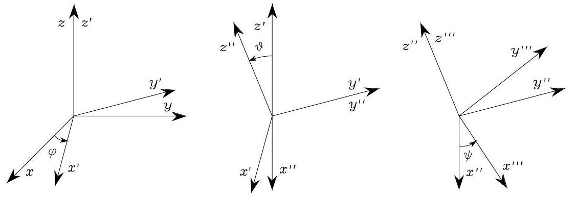
Fig. 20 ZYZ Euler angles

ZYZ Euler Angles: first, rotate the current frame by \(\varphi\) about axis \(\boldsymbol{z}\), second, rotate the current frame by \(\vartheta\) about axis \(\boldsymbol{y}^{\prime}\), and then, rotate the current frame by \(\psi\) about axis \(\boldsymbol{z}^{\prime\prime}\). Thus, the rotation matrix from ZYZ Euler angles \(\boldsymbol{\phi}=\left[\begin{array}{lll}\varphi & \vartheta & \psi\end{array}\right]^{T}\) is

\[\begin{split} \begin{aligned} \boldsymbol{R}(\boldsymbol{\phi}) & =\boldsymbol{R}_{z}(\varphi) \boldsymbol{R}_{y^{\prime}}(\vartheta) \boldsymbol{R}_{z^{\prime \prime}}(\psi) =\left[\begin{array}{ccc} c_{\varphi} c_{\vartheta} c_{\psi}-s_{\varphi} s_{\psi} & -c_{\varphi} c_{\vartheta} s_{\psi}-s_{\varphi} c_{\psi} & c_{\varphi} s_{\vartheta} \\ s_{\varphi} c_{\vartheta} c_{\psi}+c_{\varphi} s_{\psi} & -s_{\varphi} c_{\vartheta} s_{\psi}+c_{\varphi} c_{\psi} & s_{\varphi} s_{\vartheta} \\ -s_{\vartheta} c_{\psi} & s_{\vartheta} s_{\psi} & c_{\vartheta} \end{array}\right] . \end{aligned} \end{split}\]

Let’s do its inverse problem. Given any rotation matrix

\[\begin{split} \boldsymbol{R}=\left[\begin{array}{lll} r_{11} & r_{12} & r_{13} \\ r_{21} & r_{22} & r_{23} \\ r_{31} & r_{32} & r_{33} \end{array}\right] . \end{split}\]

the underlying ZYZ Euler angles \(\boldsymbol{\phi}=\left[\begin{array}{lll}\varphi & \vartheta & \psi\end{array}\right]^{T}\) is

\[\begin{split} \begin{aligned} & \varphi=\operatorname{Atan} 2\left(r_{23}, r_{13}\right) \\ & \vartheta=\operatorname{Atan} 2\left(\sqrt{r_{13}^{2}+r_{23}^{2}}, r_{33}\right) \\ & \psi=\operatorname{Atan} 2\left(r_{32},-r_{31}\right) . \end{aligned} \end{split}\]

if \(s_{\vartheta}=0\), i.e., \((r_{23}, r_{13})\not=(0,0)\); otherwise, only the sum or difference of \(\varphi\) and \(\psi\) is determined (why?)

RPY (ZYX) Euler Angles: Think about a fighter jet from parking –> taxiing (yaw) –> take-off (pitch) –> fighting (roll). RPY could be insipred by this process. Ffirst, rotate the reference frame by \(\varphi\) about the current axis \(\boldsymbol{z}\) (yaw), then, rotate the current frame by \(\vartheta\) about the current axis \(\boldsymbol{y}\) (pitch), and then, rotate the current frame by \(\psi\) about current axis \(\boldsymbol{x}\) (roll). Thus, the resulting rotation matrix is

\[\begin{split} \begin{aligned} \boldsymbol{R}(\boldsymbol{\phi}) & =\boldsymbol{R}_{z}(\varphi) \boldsymbol{R}_{y}(\vartheta) \boldsymbol{R}_{x}(\psi) =\left[\begin{array}{ccc} c_{\varphi} c_{\vartheta} & c_{\varphi} s_{\vartheta} s_{\psi}-s_{\varphi} c_{\psi} & c_{\varphi} s_{\vartheta} c_{\psi}+s_{\varphi} s_{\psi} \\ s_{\varphi} c_{\vartheta} & s_{\varphi} s_{\vartheta} s_{\psi}+c_{\varphi} c_{\psi} & s_{\varphi} s_{\vartheta} c_{\psi}-c_{\varphi} s_{\psi} \\ -s_{\vartheta} & c_{\vartheta} s_{\psi} & c_{\vartheta} c_{\psi} \end{array}\right] . \end{aligned} \end{split}\]

Inversely, given rotation matrix

\[\begin{split} \boldsymbol{R}=\left[\begin{array}{lll} r_{11} & r_{12} & r_{13} \\ r_{21} & r_{22} & r_{23} \\ r_{31} & r_{32} & r_{33} \end{array}\right], \end{split}\]

the corresponding ZYX Euler Angles is

\[\begin{split} \begin{aligned} & \varphi=\operatorname{Atan} 2\left(r_{21}, r_{11}\right) \\ & \vartheta=\operatorname{Atan} 2\left(-r_{31}, \sqrt{r_{32}^{2}+r_{33}^{2}}\right) \\ & \psi=\operatorname{Atan} 2\left(r_{32}, r_{33}\right) . \end{aligned} \end{split}\]

if \(c_{\vartheta}\not=0\); otherwise, only the sum or difference of \(\varphi\) and \(\psi\) can be determined.

Angle Axis

A rotation can also be defined by an angle \(\vartheta\) around a arbitrary unit axis \(\boldsymbol{r}=\left[r_{x}, r_{y}, r_{z}\right]^{T}\) in the reference frame \(O- x y z\), the angle-axis parameterization is written as \((\vartheta, \boldsymbol{r})\).

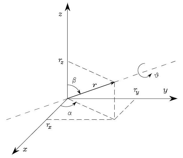
Fig. 21 Rotation of an angle about an axis.

Given the angle-axis parameterization \((\vartheta, \boldsymbol{r})\), the rotation matrix is

\[\begin{split} \boldsymbol{R}(\vartheta, \boldsymbol{r})=\left[\begin{array}{ccc} r_{x}^{2}\left(1-c_{\vartheta}\right)+c_{\vartheta} & r_{x} r_{y}\left(1-c_{\vartheta}\right)-r_{z} s_{\vartheta} & r_{x} r_{z}\left(1-c_{\vartheta}\right)+r_{y} s_{\vartheta} \\ r_{x} r_{y}\left(1-c_{\vartheta}\right)+r_{z} s_{\vartheta} & r_{y}^{2}\left(1-c_{\vartheta}\right)+c_{\vartheta} & r_{y} r_{z}\left(1-c_{\vartheta}\right)-r_{x} s_{\vartheta} \\ r_{x} r_{z}\left(1-c_{\vartheta}\right)-r_{y} s_{\vartheta} & r_{y} r_{z}\left(1-c_{\vartheta}\right)+r_{x} s_{\vartheta} & r_{z}^{2}\left(1-c_{\vartheta}\right)+c_{\vartheta} \end{array}\right] . \end{split}\]

with

\[ \begin{gathered} \sin \alpha=\frac{r_{y}}{\sqrt{r_{x}^{2}+r_{y}^{2}}} \quad \cos \alpha=\frac{r_{x}}{\sqrt{r_{x}^{2}+r_{y}^{2}}} \quad \sin \beta=\sqrt{r_{x}^{2}+r_{y}^{2}} \quad \cos \beta=r_{z} . \end{gathered} \]

Also, the following property holds:

\[ \boldsymbol{R}(-\vartheta,-\boldsymbol{r})=\boldsymbol{R}(\vartheta, \boldsymbol{r}) \]

Inversely, given rotation matrix

\[\begin{split} \boldsymbol{R}=\left[\begin{array}{lll} r_{11} & r_{12} & r_{13} \\ r_{21} & r_{22} & r_{23} \\ r_{31} & r_{32} & r_{33} \end{array}\right], \end{split}\]

then,

\[\begin{split} \begin{aligned} \vartheta=\cos ^{-1}\left(\frac{r_{11}+r_{22}+r_{33}-1}{2}\right) \quad \boldsymbol{r}=\frac{1}{2 \sin \vartheta}\left[\begin{array}{l} r_{32}-r_{23} \\ r_{13}-r_{31} \\ r_{21}-r_{12} \end{array}\right], \end{aligned} \end{split}\]

if \(\sin \vartheta \neq 0\); otherwise, \((\vartheta, \boldsymbol{r})\) is undefined.

Quaternion

From the angle-axis parameterization \((\vartheta, \boldsymbol{r})\), one can define the corresponding quaternion as

\[ \mathcal{Q}=\{\eta, \boldsymbol{\epsilon}\}, \quad\text{with} \quad \eta=\cos \frac{\vartheta}{2}, \quad \boldsymbol{\epsilon}=\sin \frac{\vartheta}{2} \boldsymbol{r} \]

\(\eta\) is called the scalar part of the quaternion, and \(\boldsymbol{\epsilon}=\left[\epsilon_{x} , \epsilon_{y} , \epsilon_{z} \right]^{T}\) is called vector part of the quaternion. Thus, we need four elements to define quaternion, but the four elements should be satisifying \(\eta^{2}+\epsilon_{x}^{2}+\epsilon_{y}^{2}+\epsilon_{z}^{2}=1\).

It is worth remarking that, unlike the angle/axis representation, a rotation by \((-\vartheta, -\boldsymbol{r})\) gives the same quaternion as that by \((\vartheta, \boldsymbol{r})\).

The rotation matrix corresponding to a given quaternion is

\[\begin{split} \boldsymbol{R}(\eta, \boldsymbol{\epsilon})=\left[\begin{array}{ccc} 2\left(\eta^{2}+\epsilon_{x}^{2}\right)-1 & 2\left(\epsilon_{x} \epsilon_{y}-\eta \epsilon_{z}\right) & 2\left(\epsilon_{x} \epsilon_{z}+\eta \epsilon_{y}\right) \\ 2\left(\epsilon_{x} \epsilon_{y}+\eta \epsilon_{z}\right) & 2\left(\eta^{2}+\epsilon_{y}^{2}\right)-1 & 2\left(\epsilon_{y} \epsilon_{z}-\eta \epsilon_{x}\right) \\ 2\left(\epsilon_{x} \epsilon_{z}-\eta \epsilon_{y}\right) & 2\left(\epsilon_{y} \epsilon_{z}+\eta \epsilon_{x}\right) & 2\left(\eta^{2}+\epsilon_{z}^{2}\right)-1 \end{array}\right] \end{split}\]

Inversely, given rotation matrix

\[\begin{split} \boldsymbol{R}=\left[\begin{array}{lll} r_{11} & r_{12} & r_{13} \\ r_{21} & r_{22} & r_{23} \\ r_{31} & r_{32} & r_{33} \end{array}\right], \end{split}\]

the quaternion is

\[\begin{split} \begin{aligned} \eta =\frac{1}{2} \sqrt{r_{11}+r_{22}+r_{33}+1} \qquad \boldsymbol{\epsilon} =\frac{1}{2}\left[\begin{array}{l} \operatorname{sgn}\left(r_{32}-r_{23}\right) \sqrt{r_{11}-r_{22}-r_{33}+1} \\ \operatorname{sgn}\left(r_{13}-r_{31}\right) \sqrt{r_{22}-r_{33}-r_{11}+1} \\ \operatorname{sgn}\left(r_{21}-r_{12}\right) \sqrt{r_{33}-r_{11}-r_{22}+1} \end{array}\right], \end{aligned} \end{split}\]

where \(\operatorname{sgn}(x)=1\) for \(x \geq 0\) and \(\operatorname{sgn}(x)=-1\) for \(x<0\).

Similar to the inverse of a rotation matrix \(\boldsymbol{R}\), a quaternion also has its own inverse, denoted as \(\mathcal{Q}^{-1}\), corresponding to \(\boldsymbol{R}^{-1}=\boldsymbol{R}^{T}\). Quanternion inverse can be easily computed as

\[ \mathcal{Q}^{-1}=\{\eta,-\boldsymbol{\epsilon}\} \]

Let \(\mathcal{Q}_{1}=\left\{\eta_{1}, \boldsymbol{\epsilon}_{1}\right\}\) and \(\mathcal{Q}_{2}=\left\{\eta_{2}, \boldsymbol{\epsilon}_{2}\right\}\) denote the quaternions corresponding to the rotation matrices \(\boldsymbol{R}_{1}\) and \(\boldsymbol{R}_{2}\), respectively. The quaternion corresponding to the product \(\boldsymbol{R}_{1} \boldsymbol{R}_{2}\) is given by

\[ \mathcal{Q}_{1} * \mathcal{Q}_{2}=\left\{\eta_{1} \eta_{2}-\boldsymbol{\epsilon}_{1}^{T} \boldsymbol{\epsilon}_{2}, \eta_{1} \boldsymbol{\epsilon}_{2}+\eta_{2} \boldsymbol{\epsilon}_{1}+\boldsymbol{\epsilon}_{1} \times \boldsymbol{\epsilon}_{2}\right\} \]

Homogeneous Transformations

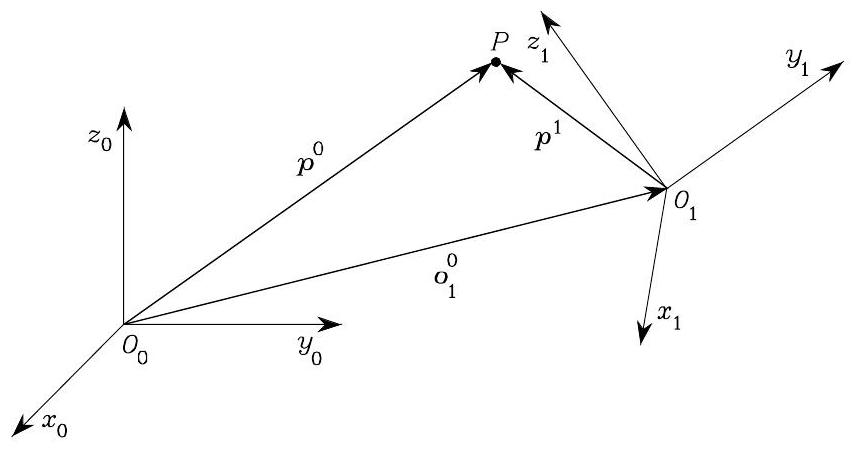
Fig. 22 Representation of a point \(P\) in different coordinate frames

Consider a reference frame \(O_{0}- x_{0} y_{0} z_{0}\) and body frame \(O_{1}- x_{1} y_{1} z_{1}\). Let \(\boldsymbol{o}_{1}^{0}\) be the coordinate of the origin of body frame in reference frame, and \(\boldsymbol{R}_{1}^{0}\) be the rotation matrix of body frame in reference frame. Let \(\boldsymbol{p}^{0}\) be the coordinate of any point \(P\) in reference frame, and \(\boldsymbol{p}^{1}\) be the coordinate of the same point \(P\) in body frame. Then, we have the following relationship

\[ \boldsymbol{p}^{0}=\boldsymbol{o}_{1}^{0}+\boldsymbol{R}_{1}^{0} \boldsymbol{p}^{1} \]

To achieve a compact notation, we first introduce the concept of “homogeneous coordinate” of a 3D vector \(\boldsymbol{p}\), defined as

\[\begin{split} \widetilde{\boldsymbol{p}}=\left[\begin{array}{l} \boldsymbol{p} \\ 1 \end{array}\right] . \end{split}\]

Then, the above relationship can be compactly written as

\[ \widetilde{\boldsymbol{p}}^{0}=\boldsymbol{T}_{1}^{0} \widetilde{\boldsymbol{p}}^{1} \]

with

\[\begin{split} \boldsymbol{T}_{1}^{0}=\left[\begin{array}{cc} \boldsymbol{R}_{1}^{0} & \boldsymbol{o}_{1}^{0} \\ \mathbf{0}^{T} & 1 \end{array}\right] \end{split}\]

which is called homogeneous transformation matrix.

The inverse of the homogeneous transformation \(\boldsymbol{T}_{1}^{0}\),

\[ \widetilde{\boldsymbol{p}}^{1}=\boldsymbol{T}_{0}^{1} \widetilde{\boldsymbol{p}}^{0}=\left(\boldsymbol{T}_{1}^{0}\right)^{-1} \widetilde{\boldsymbol{p}}^{0} \]

with

\[\begin{split} \boldsymbol{T}_{0}^{1}=\left[\begin{array}{cc} \boldsymbol{R}_{1}^{0 T} & -\boldsymbol{R}_{1}^{0 T} \boldsymbol{o}_{1}^{0} \\ \mathbf{0}^{T} & 1 \end{array}\right]=\left[\begin{array}{cc} \boldsymbol{R}_{0}^{1} & -\boldsymbol{R}_{0}^{1} \boldsymbol{o}_{1}^{0} \\ \mathbf{0}^{T} & 1 \end{array}\right]. \end{split}\]

Notice that for the homogeneous transformation matrix the orthogonality property does not hold:

\[ \boldsymbol{T}^{-1} \neq \boldsymbol{T}^{T} \]

Following the derivation of sequential rotation transformation, it is easy to verify that a sequence of homogeneous transformations can be composed by the postmultiplication rule

\[ \widetilde{\boldsymbol{p}}^{0}=\boldsymbol{T}_{1}^{0} \boldsymbol{T}_{2}^{1} \ldots \boldsymbol{T}_{n}^{n-1} \widetilde{\boldsymbol{p}}^{n} \]

where \(\boldsymbol{T}_{i}^{i-1}\) denotes the homogeneous transformation of frame \(i\) with respect to the current frame \(i-1\).