Jacobian
Notation convention warning of this lecture: if a vector has no superscript, it means this vector is expressed in the world frame by default; otherwise, the frame the coordinates of this vector is with respect to will be specified on its superscript.
Recall that FK of a \(n\) -DOF robot arm is
\[\begin{split}\boldsymbol{T}_{e}(\boldsymbol{q})=\left[\begin{array}{cc}
\boldsymbol{R}_{e}(\boldsymbol{q}) & \boldsymbol{p}_{e}(\boldsymbol{q}) \\
\mathbf{0}^{T} & 1
\end{array}\right]\end{split}\]
where the joint variable vector \(\boldsymbol{q}=\left[q_{1},\ldots, q_{n}\right]^{T}\) . The concept of
Jacobian is to the relationship between the
joint velocities and the end-effector linear and angular velocities. In
other words, we want to find the end-effector’s linear velocity
\(\dot{\boldsymbol{p}}_{e}\) and angular velocity
\(\boldsymbol{\omega}_{e}\) as a function of the joint velocities
\(\dot{\boldsymbol{q}}\) in the following form:
\[\begin{split}\begin{aligned}
& \dot{\boldsymbol{p}}_{e}=\boldsymbol{J}_{P}(\boldsymbol{q}) \dot{\boldsymbol{q}} \\
& \boldsymbol{\omega}_{e}=\boldsymbol{J}_{O}(\boldsymbol{q}) \dot{\boldsymbol{q}}
\end{aligned}\end{split}\]
Here, the matrices \(\boldsymbol{J}_{P}(\boldsymbol{q})\) and \(\boldsymbol{J}_{O}(\boldsymbol{q})\) are called linear Jacobian and angular Jacobian, respectively. Those matrices themselves are functions of \(\boldsymbol{q}\) .
In compact form, we use \(\boldsymbol{v}_{e}\) to combine the linear and angular velocities (\(\boldsymbol{v}_{e}\) is often called the twist of the end-effector):
\[\begin{split}\boldsymbol{v}_{e}=\left[\begin{array}{c}
\dot{\boldsymbol{p}}_{e} \\
\boldsymbol{\omega}_{e}
\end{array}\right]=\left[\begin{array}{l}
\boldsymbol{J}_{P}(\boldsymbol{q}) \\
\boldsymbol{J}_{O}(\boldsymbol{q})
\end{array}\right]\dot{\boldsymbol{q}}=\boldsymbol{J}(\boldsymbol{q}) \dot{\boldsymbol{q}}\end{split}\]
The stacked \((6 \times n)\) matrix \(\boldsymbol{J}(\boldsymbol{q})\) is also called geometric Jacobian.
Linear Jacobian
To compute linear Jacobian \(\boldsymbol{J}_{P}(\boldsymbol{q})\) , we can
write
\[\begin{split}\dot{\boldsymbol{p}}_{e}=\boldsymbol{J}_{P}(\boldsymbol{q}) \dot{\boldsymbol{q}}
=
\begin{bmatrix}
\boldsymbol{J}_{P,1} & \boldsymbol{J}_{P,2}& \cdots & \boldsymbol{J}_{P,n}
\end{bmatrix}
\begin{bmatrix}
\dot{q}_{1} \\ \dot{q}_{2}\\ \vdots \\ \dot{q}_{n}
\end{bmatrix}
=
\sum_{i=1}^{n} \dot{q}_{i}\boldsymbol{J}_{P,i}
\end{split}\]
Thus, \(\dot{\boldsymbol{p}}_{e}\) is
the sum of \(\dot{q}_{i} \boldsymbol{J}_{P,i}\) . Each \(\dot{q}_{i} \boldsymbol{J}_{P,i}\)
represents the contribution of the velocity of Joint \(i\) to the linear velocity of the
end-effector when all the other joints hold still.
If Joint \(i\) is prismatic,
\[\dot{q}_{i} \boldsymbol{J}_{P, i}=\dot{d}_{i} \boldsymbol{z}_{i-1}\]
and then
\[\boldsymbol{J}_{P, i}=\boldsymbol{z}_{i-1} \text {. }\]
If Joint \(i\) is revolute,
\[\dot{q}_{i} \boldsymbol{J}_{P,i}=\boldsymbol{\omega}_{i-1, i} \times \boldsymbol{r}_{i-1, e}=\dot{\vartheta}_{i} \boldsymbol{z}_{i-1} \times\left(\boldsymbol{p}_{e}-\boldsymbol{p}_{i-1}\right)\]
and then
\[\boldsymbol{J}_{P,i}=\boldsymbol{z}_{i-1} \times\left(\boldsymbol{p}_{e}-\boldsymbol{p}_{i-1}\right)\]
Angular Jacobian
To compute angular Jacobian \(\boldsymbol{J}_{O}(\boldsymbol{q})\) , we can write
\[\begin{split}\boldsymbol{\omega}_{e}
=
\begin{bmatrix}
\boldsymbol{J}_{O,1} & \boldsymbol{J}_{O,2}& \cdots & \boldsymbol{J}_{O,n}
\end{bmatrix}
\begin{bmatrix}
\dot{q}_{1} \\ \dot{q}_{2}\\ \vdots \\ \dot{q}_{n}
\end{bmatrix}=\sum_{i=1}^{n} \dot{q}_{i}\boldsymbol{J}_{O, i}
\end{split}\]
\(\dot{\boldsymbol{\omega}}_{e}\) is
the sum of the terms \(\dot{q}_{i} \boldsymbol{J}_{O,i}\) . Each \(\dot{q}_{i} \boldsymbol{J}_{O,i}\)
is the contribution of the velocity of Joint \(i\) to the angular velocity of the
end-effector when all the other joints hold still.
If Joint \(i\) is prismatic, it is
\[\dot{q}_{i} \boldsymbol{J}_{O,i}=\mathbf{0}\]
and then
\[\boldsymbol{J}_{O,i}=\mathbf{0}\]
If Joint \(i\) is revolute, it is
\[\dot{q}_{i} \boldsymbol{J}_{O,i}=\dot{\vartheta}_{i} \boldsymbol{z}_{i-1}\]
and then
\[\boldsymbol{J}_{O,i}=\boldsymbol{z}_{i-1}\]
Summary
Important
In summary, the velocity (twist) of the end-effector is
\[\begin{split}\boldsymbol{v}_e=\boldsymbol{J}(\boldsymbol{q})\boldsymbol{\dot{q}}=
\begin{bmatrix}
\boldsymbol{J}_{P,1} & \boldsymbol{J}_{P,2}& \cdots & \boldsymbol{J}_{P,n}\\
\boldsymbol{J}_{O,1} & \boldsymbol{J}_{O,2}& \cdots & \boldsymbol{J}_{O,n}
\end{bmatrix}
\begin{bmatrix}
\dot{q}_{1} \\ \dot{q}_{2}\\ \vdots \\ \dot{q}_{n}
\end{bmatrix}
\end{split}\]
Here, Jacobian is
\[\begin{split}\boldsymbol{J}(\boldsymbol{q})=
\begin{bmatrix}
\boldsymbol{J}_{P,1} & \boldsymbol{J}_{P,2}& \cdots & \boldsymbol{J}_{P,n}\\
\boldsymbol{J}_{O,1} & \boldsymbol{J}_{O,2}& \cdots & \boldsymbol{J}_{O,n}
\end{bmatrix}
\
\end{split}\]
For the \(i\) -th column, if the joint \(i\) is prismatic, then
(19) \[\begin{split}
\begin{bmatrix}
\boldsymbol{J}_{P,i} \\
\boldsymbol{J}_{O,i}
\end{bmatrix}
= \begin{bmatrix}
\boldsymbol{z}_{i-1} \\
\mathbf{0}
\end{bmatrix}
\end{split}\]
if the joint \(i\) is revolute joint, then
(20) \[\begin{split}
\begin{bmatrix}
\boldsymbol{J}_{P,i} \\
\boldsymbol{J}_{O,i}
\end{bmatrix}
= \begin{bmatrix}
\boldsymbol{z}_{i-1} \times\left(\boldsymbol{p}_{e}-\boldsymbol{p}_{i-1}\right) \\
\boldsymbol{z}_{i-1}
\end{bmatrix}
\end{split}\]
In above (19) or (20) ,
\(\boldsymbol{z}_{i-1}, \boldsymbol{p}_{e}\) and \(\boldsymbol{p}_{i-1}\)
can be obtained from FK.
Examples
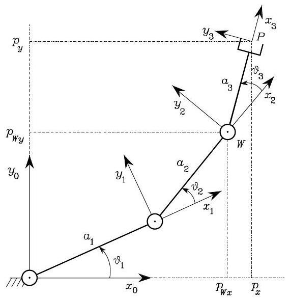
Three-link Planar Arm
The Jacobian formula is
\[\begin{split}\boldsymbol{J}(\boldsymbol{q})=\left[\begin{array}{ccc}
\boldsymbol{z}_{0} \times\left(\boldsymbol{p}_{3}-\boldsymbol{p}_{0}\right) & \boldsymbol{z}_{1} \times\left(\boldsymbol{p}_{3}-\boldsymbol{p}_{1}\right) & \boldsymbol{z}_{2} \times\left(\boldsymbol{p}_{3}-\boldsymbol{p}_{2}\right) \\
\boldsymbol{z}_{0} & \boldsymbol{z}_{1} & \boldsymbol{z}_{2}
\end{array}\right]\end{split}\]
From the forward kinematics, we have
\[\begin{split}\boldsymbol{p}_{0}=\left[\begin{array}{l}
0 \\
0 \\
0
\end{array}\right] \quad \boldsymbol{p}_{1}=\left[\begin{array}{c}
a_{1} c_{1} \\
a_{1} s_{1} \\
0
\end{array}\right] \quad \boldsymbol{p}_{2}=\left[\begin{array}{c}
a_{1} c_{1}+a_{2} c_{12} \\
a_{1} s_{1}+a_{2} s_{12} \\
0
\end{array}\right]
\quad
\boldsymbol{p}_{3}=\left[\begin{array}{c}
a_{1} c_{1}+a_{2} c_{12}+a_{3} c_{123} \\
a_{1} s_{1}+a_{2} s_{12}+a_{3} s_{123} \\
0
\end{array}\right]\end{split}\]
and
\[\begin{split}\boldsymbol{z}_{0}=\boldsymbol{z}_{1}=\boldsymbol{z}_{2}=\left[\begin{array}{l}
0 \\
0 \\
1
\end{array}\right]\end{split}\]
Then, assembly the Jacobian matricx
\[\begin{split}\boldsymbol{J}=\left[\begin{array}{ccc}
-a_{1} s_{1}-a_{2} s_{12}-a_{3} s_{123} & -a_{2} s_{12}-a_{3} s_{123} & -a_{3} s_{123} \\
a_{1} c_{1}+a_{2} c_{12}+a_{3} c_{123} & a_{2} c_{12}+a_{3} c_{123} & a_{3} c_{123} \\
0 & 0 & 0 \\
0 & 0 & 0 \\
0 & 0 & 0 \\
1 & 1 & 1
\end{array}\right]\end{split}\]
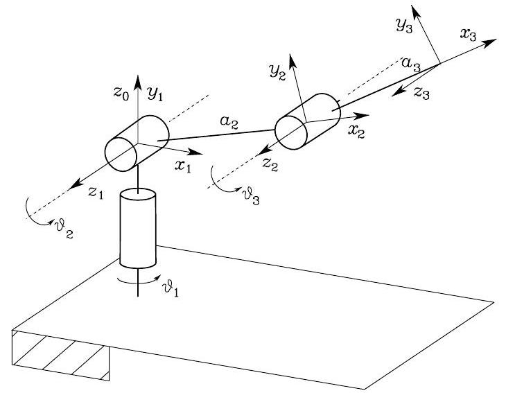
Anthropomorphic Arm
The Jacobian formula is
\[\begin{split}\boldsymbol{J}=\left[\begin{array}{ccc}
\boldsymbol{z}_{0} \times\left(\boldsymbol{p}_{3}-\boldsymbol{p}_{0}\right) & \boldsymbol{z}_{1} \times\left(\boldsymbol{p}_{3}-\boldsymbol{p}_{1}\right) & \boldsymbol{z}_{2} \times\left(\boldsymbol{p}_{3}-\boldsymbol{p}_{2}\right) \\
\boldsymbol{z}_{0} & \boldsymbol{z}_{1} & \boldsymbol{z}_{2}
\end{array}\right]\end{split}\]
From FK, we have
\[\begin{split}\begin{gathered}
\boldsymbol{p}_{0}=\boldsymbol{p}_{1}=\left[\begin{array}{l}
0 \\
0 \\
0
\end{array}\right] \quad \boldsymbol{p}_{2}=\left[\begin{array}{c}
a_{2} c_{1} c_{2} \\
a_{2} s_{1} c_{2} \\
a_{2} s_{2}
\end{array}\right] \quad
\boldsymbol{p}_{3}=\left[\begin{array}{c}
c_{1}\left(a_{2} c_{2}+a_{3} c_{23}\right) \\
s_{1}\left(a_{2} c_{2}+a_{3} c_{23}\right) \\
a_{2} s_{2}+a_{3} s_{23}
\end{array}\right]
\end{gathered}\end{split}\]
and
\[\begin{split}\boldsymbol{z}_{0}=\left[\begin{array}{l}
0 \\
0 \\
1
\end{array}\right] \quad \boldsymbol{z}_{1}=\boldsymbol{z}_{2}=\left[\begin{array}{c}
s_{1} \\
-c_{1} \\
0
\end{array}\right]\end{split}\]
Then,
\[\begin{split}\boldsymbol{J}=\left[\begin{array}{ccc}
-s_{1}\left(a_{2} c_{2}+a_{3} c_{23}\right) & -c_{1}\left(a_{2} s_{2}+a_{3} s_{23}\right) & -a_{3} c_{1} s_{23} \\
c_{1}\left(a_{2} c_{2}+a_{3} c_{23}\right) & -s_{1}\left(a_{2} s_{2}+a_{3} s_{23}\right) & -a_{3} s_{1} s_{23} \\
0 & a_{2} c_{2}+a_{3} c_{23} & a_{3} c_{23} \\
0 & s_{1} & s_{1} \\
0 & -c_{1} & -c_{1} \\
1 & 0 & 0
\end{array}\right]\end{split}\]
Analytical Jacobian (Optional)
The above derived Jacobian is a mapping from joint velocities to the
end-effector’s linear and angular velocity
\[\begin{split}\boldsymbol{v}_{e}=\left[\begin{array}{c}
\dot{\boldsymbol{p}}_{e} \\
\boldsymbol{\omega}_{e}
\end{array}\right]=\boldsymbol{J}(\boldsymbol{q}) \dot{\boldsymbol{q}}\end{split}\]
If the end-effector’s orientation is specified in terms of a minimal number of
parameters instead of rotation matrix, say
\[\begin{split}{\boldsymbol{x}}_{e}=\left[\begin{array}{c}
{\boldsymbol{p}}_{e} \\
{\boldsymbol{\phi}}_{e}
\end{array}\right]\end{split}\]
we need to find a Jacobian
\[\begin{split}\dot{\boldsymbol{x}}_{e}=\left[\begin{array}{c}
\dot{\boldsymbol{p}}_{e} \\
\dot{\boldsymbol{\phi}}_{e}
\end{array}\right]
=
\begin{bmatrix}
\boldsymbol{J}_{P}(\boldsymbol{q})\\
\boldsymbol{J}_{\phi}(\boldsymbol{q})
\end{bmatrix}
\dot{\boldsymbol{q}}
\end{split}\]
Here, the linear Jacobian remains the same as before, the only difference is the angular Jacobian \(\boldsymbol{J}_{O}(\boldsymbol{q})\) becomes
\[
\dot{\boldsymbol{\phi}}_{e}=
\boldsymbol{J}_{\phi}(\boldsymbol{q}) \dot{\boldsymbol{q}}
\]
We call the new Jacobian matrix
\[\begin{split}
\boldsymbol{J}_{A}(\boldsymbol{q})=\begin{bmatrix}
\boldsymbol{J}_{P}(\boldsymbol{q})\\
\boldsymbol{J}_{\phi}(\boldsymbol{q})
\end{bmatrix}
\end{split}\]
the analytical Jacobian (recall \(\boldsymbol{J}\) is called geometrical Jacobian or Jacobian).
How do we find \(\boldsymbol{J}_{A}(\boldsymbol{q})\) from \(\boldsymbol{J}\) ? To do so, we need a mapping
\[\begin{split}\left[\begin{array}{c}
\dot{\boldsymbol{p}}_{e} \\
\boldsymbol{\omega}_{e}
\end{array}\right] = \underbrace{\begin{bmatrix}
\boldsymbol{I} & \boldsymbol{0} \\
\boldsymbol{0} & \boldsymbol{N}\left(\phi_{e}\right)
\end{bmatrix}}_{\boldsymbol{T}}
\left[\begin{array}{c}
\dot{\boldsymbol{p}}_{e} \\
\dot{\boldsymbol{\phi}}_{e}
\end{array}\right]\end{split}\]
such that
\[\boldsymbol{J}_{A}(\boldsymbol{q}) = \boldsymbol{T}^{-1} \boldsymbol{J}(\boldsymbol{q})\]
In the following, we will find out the mapping
\[\boldsymbol{\omega}_{e}=\boldsymbol{N}\left(\phi_{e}\right)\dot{\boldsymbol{\phi}}_{e}\]
for the Euler ZYZ Angle
\({\boldsymbol{\phi}}_{e}=[{\varphi}, {\vartheta}, \psi]^T\) .
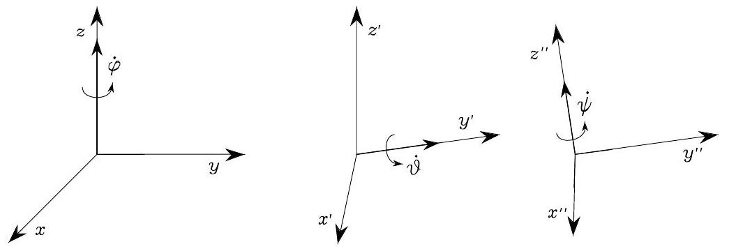
Recall the rotation induced from the Euler ZYZ Angle. The angualr velocities \(\dot{\varphi}, \dot{\vartheta}, \dot\psi\) is always with respect to the current frame, as shown in Fig. 54
Fig. 54 Rotational velocities of Euler angles ZYZ in current
frame
Therefore, to compute \(\boldsymbol{\omega}_{e}\) , we just need to first, express each Euler angle velocity \(\dot{\varphi}, \dot{\vartheta}, \dot\psi\) from its respective current from to the reference
frame, and second, sum them up!
\[\dot{\varphi}\left[\begin{array}{lll}0 & 0 & 1\end{array}\right]^{T}\]
\[\dot{\vartheta}\left[\begin{array}{lll}-s_{\varphi} & c_{\varphi} & 0\end{array}\right]^{T}\]
\[\dot{\psi}\left[\begin{array}{lll}c_{\varphi} s_{\vartheta} & s_{\varphi} s_{\vartheta} & c_{\vartheta}\end{array}\right]^{T}\]
Thus,
\[\begin{split}\boldsymbol{N}\left(\phi_{e}\right) =\left[\begin{array}{ccc}
0 & -s_{\varphi} & c_{\varphi} s_{\vartheta} \\
0 & c_{\varphi} & s_{\varphi} s_{\vartheta} \\
1 & 0 & c_{\vartheta}
\end{array}\right] .\end{split}\]