Singularity & Redundancy

The Jacobian of a robot arm is defined as

\[\boldsymbol{v}_{e}=\boldsymbol{J}(\boldsymbol{q}) \dot{\boldsymbol{q}}\]

between joint velocity \(\dot{\boldsymbol{q}}\) and the end-effector velocity \(\boldsymbol{v}_{e}=\left[\begin{array}{ll}\dot{\boldsymbol{p}}_{e}^{T} & \boldsymbol{\omega}_{e}^{T}\end{array}\right]^{T}\). Jacobian is a function of the configuration \(\boldsymbol{q}\). We call the configurations \(\boldsymbol{q}\) at which \(\boldsymbol{J}(\boldsymbol{q})\) is rank-deficient as singularity. Or, we say the robot is at singularity.

Formally, for a non-redundant (\(n=r\)) or redundant (\(n> r\)) robot arm (\(r\) is the dimension of the end-effector task space, \(n\) is the dimension of the joint space), a singularity occurs when the Jacobian matrix \(\boldsymbol{J}(\boldsymbol{q})\) loses ranks:

\[ \text{rank}(\boldsymbol{J}(\boldsymbol{q})) < r\]

Here are reasons why we need to care about singularities?

• Singularities represent robot configurations at which mobility of the robot end-effector is reduced.

• Near a singularity, small velocities in the operational space (end-effector) can correspond to large velocities in the joint space.

Singularity Decoupling

Computing singularity configurations based on definition (i.e. find \(\boldsymbol{q}\) such that \( \text{rank}(\boldsymbol{J}(\boldsymbol{q})) < m\)) can be complex. However, for robot arms having a spherical wrist, it is possible to decouple the computation into two subproblems: (1) find arm singularities for the first 3 (or more) joints, and (2) find of wrist singularities for the wrist joints (last three joints).

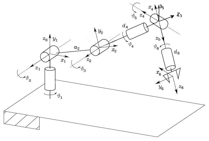
Let’s see an example of a non-redundant (\(r=n=6\)) robot arm. Consider a \(6\)-DoF robot arm (anthropomorphic robot arm) in Fig. 55, where the last 3 joints are revolute (e.g., a spherical wrist). Note that the Frame 6 is the end-effector frame \(\boldsymbol{p}_{6}=\boldsymbol{p}_{e}\).

Fig. 55 Anthropomorphic robot arm

The Jacobian can be partitioned into \((2 \times 2)\) block matrix

\[\begin{split}\boldsymbol{J}=\left[\begin{array}{ll} \boldsymbol{J}_{11} & \boldsymbol{J}_{12} \\ \boldsymbol{J}_{21} & \boldsymbol{J}_{22} \end{array}\right]\end{split}\]

with

\[\begin{split}\begin{equation} \begin{aligned} \boldsymbol{J}_{11}&=\left[\begin{array}{ccc} \boldsymbol{z}_{0} \times\left(\boldsymbol{p}_{e}-\boldsymbol{p}_{0}\right) & \boldsymbol{z}_{1} \times\left(\boldsymbol{p}_{e}-\boldsymbol{p}_{1}\right) & \boldsymbol{z}_{2}\times \left(\boldsymbol{p}_{e}-\boldsymbol{p}_{0}\right) \end{array}\right] \\ \boldsymbol{J}_{21}&=\left[\begin{array}{lll} \boldsymbol{z}_{0} & \boldsymbol{z}_{1} & \boldsymbol{z}_{2} \end{array}\right] \\ \boldsymbol{J}_{12}&=\left[\begin{array}{ccc} \boldsymbol{z}_{3} \times\left(\boldsymbol{p}_{e}-\boldsymbol{p}_{3}\right) & \boldsymbol{z}_{4} \times\left(\boldsymbol{p}_{e}-\boldsymbol{p}_{4}\right) & \boldsymbol{z}_{5} \times\left(\boldsymbol{p}_{e}-\boldsymbol{p}_{5}\right) \end{array}\right] \\ \boldsymbol{J}_{22}&=\left[\begin{array}{lll} \boldsymbol{z}_{3} & \boldsymbol{z}_{4} & \boldsymbol{z}_{5} \end{array}\right] \end{aligned} \end{equation}\end{split}\]

Because \(\boldsymbol{p}_3=\boldsymbol{p}_4=\boldsymbol{p}_5\) (i.e., the Frames 3, 4, 5 share the same origin), we can conduct row operations by multiple second row block matrices with \(\left(\boldsymbol{p}_{e}-\boldsymbol{p}_{3}\right)\) and subtract from the first row block matrices. Thus, we obtain

\[\begin{split}\boldsymbol{\bar{J}}=\left[\begin{array}{ll} \boldsymbol{\bar{J}}_{11} & \boldsymbol{0} \\ \boldsymbol{\bar{J}}_{21} & \boldsymbol{\bar{J}}_{22} \end{array}\right]\end{split}\]

\[\begin{split}\begin{equation} \begin{aligned} \boldsymbol{\bar{J}}_{11}&=\left[\begin{array}{ccc} \boldsymbol{z}_{0} \times\left(\boldsymbol{p}_{3}-\boldsymbol{p}_{0}\right) & \boldsymbol{z}_{1} \times\left(\boldsymbol{p}_{3}-\boldsymbol{p}_{1}\right) & \boldsymbol{z}_{2}\times \left(\boldsymbol{p}_{3}-\boldsymbol{p}_{1}\right) \end{array}\right] \\ \boldsymbol{\bar{J}}_{21}&=\left[\begin{array}{lll} \boldsymbol{z}_{0} & \boldsymbol{z}_{1} & \boldsymbol{z}_{2} \end{array}\right] \\ \boldsymbol{\bar{J}}_{22}&=\left[\begin{array}{lll} \boldsymbol{z}_{3} & \boldsymbol{z}_{4} & \boldsymbol{z}_{5} \end{array}\right] \end{aligned} \end{equation}\end{split}\]

Since the above row operations maintain the matrix rank and determinant, we can find the singularity by solving

\[\operatorname{det}\left(\boldsymbol{{J}}_{}\right)=\operatorname{det}\left(\boldsymbol{\bar{J}}_{}\right)=\operatorname{det}\left(\boldsymbol{\bar{J}}_{11}\right)\operatorname{det}\left(\boldsymbol{\bar{J}}_{22}\right)=0\]

Thus, singularity decoupling is achieved: we can use \(\operatorname{det}\left(\boldsymbol{\bar{J}}_{11}\right)=0\) and \(\operatorname{det}\left(\boldsymbol{\bar{J}}_{22}\right)=0\) to determine the arm singularities and wrist singularities, respectively.

Wrist Singularity

Wrist singularities can be computed by inspecting

\[ \operatorname{det}\left(\boldsymbol{\bar{J}}_{22}\right)=0 \]

Fig. 56 Spherical wrist at a singularity

In fact, the wrist is at singularity whenever the unit vectors \(\boldsymbol{z}_{3}, \boldsymbol{z}_{4}, \boldsymbol{z}_{5}\) are linearly dependent. The wrist structure shows that this occurs when \(\boldsymbol{z}_{3}\) and \(\boldsymbol{z}_{5}\) are aligned, which is shown in Fig. 56. That is,

\[\vartheta_{5}=0 \quad \text{or}\quad \vartheta_{5}=\pi\]

At wrist singularity, the end-effector loses the rotation mobility about a axis orthogonal to \(\boldsymbol{z}_{4}\) and \(\boldsymbol{z}_{3}\).

Arm Singularity

Arm singularities can be computed by inspecting

\[ \operatorname{det}\left(\boldsymbol{\bar{J}}_{11}\right)=0 \]

Consider the anthropomorphic arm in Fig. 55.

\[\operatorname{det}\left(\boldsymbol{\bar{J}}_{11}\right)=-a_{2} a_{3} s_{3}\left(a_{2} c_{2}+a_{3} c_{23}\right)\]

The determinant vanishes if \(s_{3}=0\) or \(\left(a_{2} c_{2}+a_{3} c_{23}\right)=\) 0.

The case \(s_{3}=0\) is called elbow singularity. This means that

\[\vartheta_{3}=0 \quad \text{or}\quad \vartheta_{3}=\pi\]

showing that the elbow is outstretched or retracted, as in Fig. 57. In this singularity, the end-effector will lose the linear motion along the direction of the third link (i.e., the direction perpendicular to \(\boldsymbol{z}_2\) and \(\boldsymbol{z}_0\)).

Fig. 57 Anthropomorphic arm at an elbow singularity

The case \(\left(a_{2} c_{2}+a_{3} c_{23}\right)=0\) indicates that the wrist point lies on axis \(z_{0}\), as shown in Fig. 58. This is called shoulder singularity. In this singularity, the end-effector loses the linear motion along the \(z_{1}\) direction.

Fig. 58 Anthropomorphic arm at a shoulder singularity

Redundancy

The Jacobian defines a linear mapping from the joint velocity space to the end-effector velocity space:

(21)\[\boldsymbol{v}_{e}=\boldsymbol{J}(\boldsymbol{q}) \dot{\boldsymbol{q}}\]

where \(\boldsymbol{v}_{e}\) is the \((r \times 1)\) vector of end-effector velocity; \(\dot{\boldsymbol{q}}\) is the \((n \times 1)\) vector of joint velocities; and \(\boldsymbol{J}\) is \((r \times n)\) matrix. If \(r<n\), the robot arm is kinematically redundant and there exist \((n-r)\) redundant DOFs.

Fig. 59 Mapping between the joint velocity space and the end-effector velocity space

Let’s now abstract (21) from the perspective of linear algebra, as shown in Fig. 59.

• The range of \(\boldsymbol{J}\) is the subspace \(\mathcal{R}(\boldsymbol{J})\subseteq \mathbb{R}^r\) of the end-effector velocities that can be generated by the joint velocities.

• The null space of \(\boldsymbol{J}\) is the subspace \(\mathcal{N}(\boldsymbol{J})\subseteq \mathbb{R}^n\) of the joint velocities that do not produce any end-effector velocity.

If the Jacobian has full rank at configuration \(\boldsymbol{q}\), one has

\[\operatorname{dim}(\mathcal{R}(\boldsymbol{J}))=r \quad \operatorname{dim}(\mathcal{N}(\boldsymbol{J}))=n-r\]

and the range of \(\boldsymbol{J}\) spans the entire space \(\mathbb{R}^{r}\). This means that we can theoretically command the velocity of joints to generate any end-effector velocity we want at configuration \(\boldsymbol{q}\).

Otherwise, if the Jacobian is rank-deficient at configuration \(\boldsymbol{q}\), i.e., the robot arm is a singularity at \(\boldsymbol{q}\), the dimension of the range space decreases while the dimension of the null space increases, but they must satisify (recall linear algebra)

\[\operatorname{dim}(\mathcal{R}(\boldsymbol{J}))+\operatorname{dim}(\mathcal{N}(\boldsymbol{J}))=n\]

This means that there is a set of end-effector velocities which we will never be able to generate no matter what velocity of joints we command at configuration \(\boldsymbol{q}\).

If \(\mathcal{N}(\boldsymbol{J}) \neq \emptyset\), we can find a \((n \times n)\) projection matrix \(\boldsymbol{P}\) for the null space of \(\boldsymbol{J}\), that is, the range of this projection matrix \(\boldsymbol{P}\) equals the null space of \(\boldsymbol{J}\):

\[\mathcal{R}(\boldsymbol{P}) \equiv \mathcal{N}(\boldsymbol{J})\]

The projection matrix \(\boldsymbol{P}\) has the closed-form solution:

\[ \boldsymbol{P}=\boldsymbol{I}-\boldsymbol{J}^T(\boldsymbol{J}\boldsymbol{J}^T)^{{\dagger}}\boldsymbol{J} \]

where \(\boldsymbol{I}\) is \(n\times n\) identity, and \(A^{\dagger}\) is the Moore–Penrose pseudoinverse of \(A\).