Joint Space Control

Joint Space Control#

Overview of Robot Control#

The control of a robot arm is to determine the time sequence of control inputs (i.e., joint torques) to achieve a specified task. A task is specified usually in the operational space (such as end-effector motion and forces), whereas control inputs (joint torque) is usually made in the joint space. There are two control schemes: joint space control and operational space control.

../_images/joint_control.jpg — Fig. 65 Joint space control#

The joint space control is shown in Fig. 65. Here, inverse kinematics is use to convert the specified end-effector motion \(\boldsymbol{x}_{d}\) to the desired joint motion \(\boldsymbol{q}_{d}\). Then, a joint space controller is designed to allow the actual joint value \(\boldsymbol{q}\) to track \(\boldsymbol{q}_{d}\). The controller directly regulates the joint tracking error \(\boldsymbol{q}_{d}-\boldsymbol{q}_{}\), instead of operational space error \(\boldsymbol{x}_{d}-\boldsymbol{x}_{e}\). Thus, the end-effector pose \(\boldsymbol{x}_{e}\) is controlled in an open-loop fashion.

../_images/operational_space_control.jpg — Fig. 66 Operational space control#

The operational space control is shown in Fig. 66. Here, the operational space motion \(\boldsymbol{x}_{e}\) is directly fed back to the controller. Thus, it addresses the drawbacks of joint space control. However, the control typically is more complex in design and requires measuring the operational space motion \(\boldsymbol{x}_{e}\).

Joint Space Control#

For a \(n\)-joint robot arm, we consider a robot arm without external end-effector forces and joint friction. The equation of motion of the robot arm is

(51)#\[ \boldsymbol{B}(\boldsymbol{q}) \ddot{\boldsymbol{q}}+\boldsymbol{C}(\boldsymbol{q}, \dot{\boldsymbol{q}}) \dot{\boldsymbol{q}}+\boldsymbol{g}(\boldsymbol{q})=\boldsymbol{\tau}.\]

The controller we want to design is

(52)#\[ \boldsymbol{\tau}=\boldsymbol{u}=\textbf{controller}(\boldsymbol{q}, \boldsymbol{\dot{q}}, \boldsymbol{q}_d, \boldsymbol{\dot{q}}_d)\]

i.e., the controller takes the robot current joint position \(\boldsymbol{q}\), joint velocity \(\boldsymbol{\dot{q}}\), desired joint position \(\boldsymbol{q}_d\), and desired joint velocity \(\boldsymbol{\dot{q}}_d\), and outputs joint torque \(\boldsymbol{u}\).

The motion of equation of the robot arm with the controller is (also called closed-loop dynamics):

(57)#\[ \boldsymbol{B}(\boldsymbol{q}) \ddot{\boldsymbol{q}}+\boldsymbol{C}(\boldsymbol{q}, \dot{\boldsymbol{q}}) \dot{\boldsymbol{q}}+\boldsymbol{g}(\boldsymbol{q})=\textbf{controller}(\boldsymbol{q}, \boldsymbol{\dot{q}}, \boldsymbol{q}_d, \boldsymbol{\dot{q}}_d)\]

Controller 1: PD Control with Gravity Compensation#

Consider a stationary desired joint position \(\boldsymbol{q}_{d}\) (\(\boldsymbol{\dot q}_{d}=\boldsymbol{0}\)), we want to design a controller (52), such that given any initial robot pose, say \(\boldsymbol{q}_0\), the controlled robot arm (57) will eventually reach \(\boldsymbol{q}_{d}\). In other words, if we define the joint error as

\[{\boldsymbol{e}}=\boldsymbol{q}_{d}-\boldsymbol{q}\]

we want to design a controller \( \boldsymbol{u}=\textbf{controller}(\boldsymbol{q}, \boldsymbol{\dot{q}}, \boldsymbol{q}_d, \boldsymbol{\dot{q}}_d)\) such that

\[\boldsymbol{e}(t)\rightarrow \boldsymbol{0}\quad \text{as}\quad t\rightarrow \infty.\]

PD Controller with Gravity Compensation

Controller for PD control with gravity compensation follows

(54)#\[ \boldsymbol{u}=\underbrace{\boldsymbol{g}(\boldsymbol{q})}_{\text{gravitational compensation}}+\underbrace{\boldsymbol{K}_{P} (\boldsymbol{q}_d-\boldsymbol{q})}_{\text{proportional control}}\quad\underbrace{-\boldsymbol{K}_{D} \dot{\boldsymbol{q}}}_{\text{derivative control}}\]

with \(\boldsymbol{K}_{P}\) and \(\boldsymbol{K}_{D}\) are positive definite matrices.

Below, we will use the Lyapunov method (see background of Lyapunov method in Numerical Inverse Kinematics) to prove that the controller (54) works.

Lyapunov stability proof for PD controller (click to expand)

First, we define the error state vector \(\begin{bmatrix}\boldsymbol{e}\\ \boldsymbol{\dot{q}}\end{bmatrix}\), and choose the following Lyapunov function:

\[\begin{split}V({\boldsymbol{e}},\dot{\boldsymbol{q}})=\frac{1}{2} \dot{\boldsymbol{q}}^{T} \boldsymbol{B}(\boldsymbol{q}) \dot{\boldsymbol{q}}+\frac{1}{2} {\boldsymbol{e}}^{T} \boldsymbol{K}_{P} {\boldsymbol{e}} \quad >0 \quad \forall \begin{bmatrix}\boldsymbol{e}\\ \boldsymbol{\dot{q}}\end{bmatrix} \neq \mathbf{0}\end{split}\]

where \(\boldsymbol{K}_{P}\) is an \((n \times n)\) symmetric positive definite matrix.

Differentiating \(V({\boldsymbol{e}},\dot{\boldsymbol{q}})\) with respect to time yields

(55)#\[\dot{V}=\dot{\boldsymbol{q}}^{T} \boldsymbol{B}(\boldsymbol{q}) \ddot{\boldsymbol{q}}+\frac{1}{2} \dot{\boldsymbol{q}}^{T} \dot{\boldsymbol{B}}(\boldsymbol{q}) \dot{\boldsymbol{q}}-\dot{\boldsymbol{q}}^{T} \boldsymbol{K}_{P} {\boldsymbol{e}}\]

From (51), we can solve for \(\boldsymbol{B} \ddot{\boldsymbol{q}}\) and substituting it to (55) gives

(56)#\[\label{equ.lypuanovdot} \dot{V}=\frac{1}{2} \underbrace{\dot{\boldsymbol{q}}^{T}(\dot{\boldsymbol{B}}(\boldsymbol{q})-2 \boldsymbol{C}(\boldsymbol{q}, \dot{\boldsymbol{q}})) \dot{\boldsymbol{q}}}_{0}+\dot{\boldsymbol{q}}^{T}\left(\boldsymbol{u}-\boldsymbol{g}(\boldsymbol{q})-\boldsymbol{K}_{P} {\boldsymbol{e}}\right)\]

The first term is zero since \(\dot{\boldsymbol{B}}-2 \boldsymbol{C}\) is a skew-symmetric matrix (see in the property of dynamics in Dynamics). For the second term, we substitute the controller (54) in, and this leads to

\[\dot{V}=-\boldsymbol{\dot{q}}^T\boldsymbol{K}_D\boldsymbol{\dot{q}} \quad <0 \quad \forall \dot{\boldsymbol{q}} \neq \mathbf{0}\]

and thus, \(V\) decreases as long as \(\dot{\boldsymbol{q}} \neq \mathbf{0}\). Thus, the robot arm will reach an equilibrium configuration where \(\dot{\boldsymbol{q}}=\mathbf{0}\). To find the equilibrium configuration, we look at the closed-loop dynamics under control

(57)#\[\boldsymbol{B}(\boldsymbol{q}) \ddot{\boldsymbol{q}}+\boldsymbol{C}(\boldsymbol{q}, \dot{\boldsymbol{q}}) \dot{\boldsymbol{q}}+\boldsymbol{g}(\boldsymbol{q})=\boldsymbol{g}(\boldsymbol{q})+\boldsymbol{K}_{P} {\boldsymbol{e}}-\boldsymbol{K}_{D} \dot{\boldsymbol{q}}\]

With \(\dot{\boldsymbol{q}}=\mathbf{0}\), it follows that \(\ddot{\boldsymbol{q}} =\mathbf{0}\), and then from the above dynamics (57), we have

\[\boldsymbol{K}_{P} {\boldsymbol{e}}=\mathbf{0} \quad\rightarrow\quad {\boldsymbol{e}}=\boldsymbol{q}_{d}-\boldsymbol{q} = \mathbf{0}\]

Therefore, the robot arm will eventually reach equilibrium, which is exactly the desired configuration \(\boldsymbol{q}_{d}\).

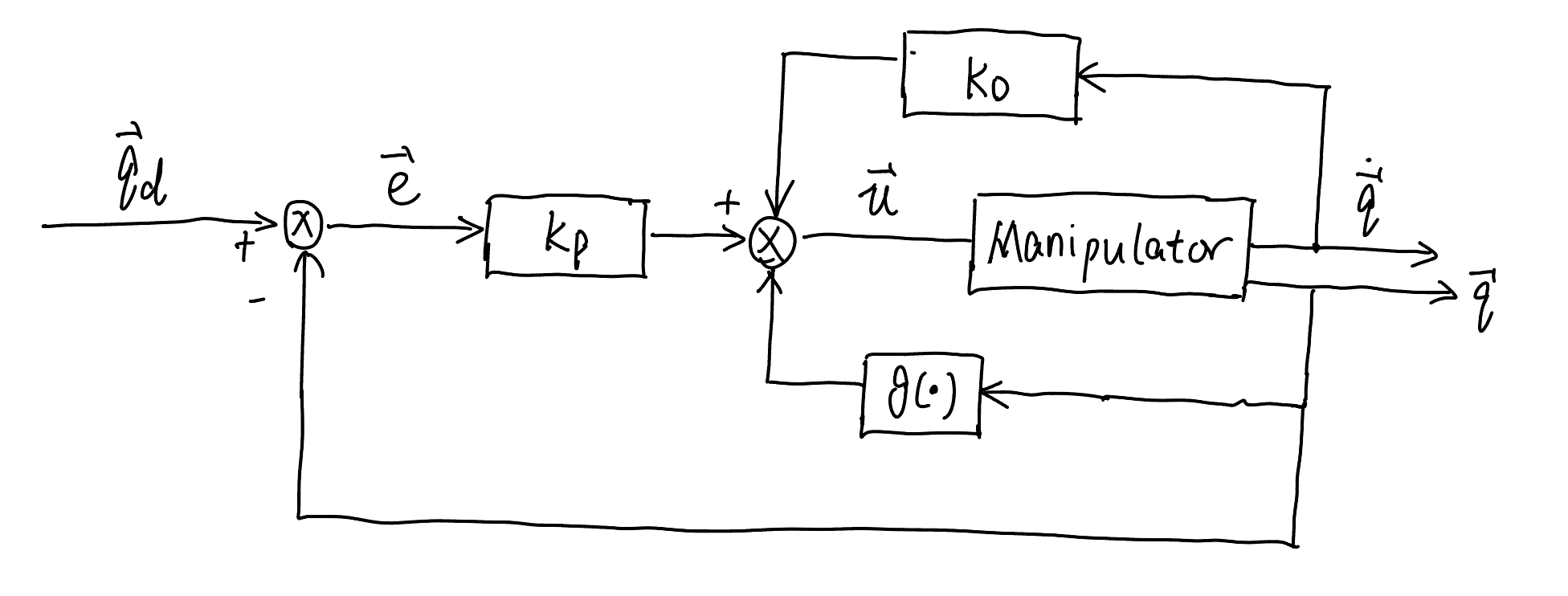
The control block diagram for PD control with gravity compensation is shown below

../_images/PD_control_with_gravity_compensation.jpeg — Fig. 67 Control diagram of PD control with gravity compensation#

Controller 2: Inverse Dynamics Control#

One limitation of the PD Control with Gravity Compensation is that the controller can only follow a stationary desired \(\boldsymbol{q}_d\), not good at tracking a fast-changing desired joint:

(58)#\[ \boldsymbol{\dot{q}}_d(t)\neq\boldsymbol{0} \quad \text{and} \quad \boldsymbol{\ddot{q}}_d(t)\neq\boldsymbol{0}\]

Inverse dynamics control is to address the above limitation. The idea of inverse dynamics control is to find a controller (52) that can make the robot arm behave like a mass-spring-damper system.

Inverse Dynamics Control

Controller for inverse dynamics control follows

(59)#\[ \boldsymbol{u}=\boldsymbol{B}(\boldsymbol{q}) \boldsymbol{y}+\boldsymbol{C}(\boldsymbol{q}, \dot{\boldsymbol{q}}) \dot{\boldsymbol{q}}+\boldsymbol{g}(\boldsymbol{q})\]

with

(60)#\[ \boldsymbol{y}=\ddot{\boldsymbol{{q}}}_d+\boldsymbol{K}_{P} ({\boldsymbol{q}}_{d}-\boldsymbol{q})+\boldsymbol{K}_{D} (\dot{\boldsymbol{q}}_{d}-\dot{\boldsymbol{q}})\]

Here,

\[ \boldsymbol{K}_{P}=\operatorname{diag}\left\{\omega_{1}^{2}, \ldots, \omega_{n}^{2}\right\} \quad \boldsymbol{K}_{D}=\operatorname{diag}\left\{2 \zeta_{1} \omega_{1}, \ldots, 2 \zeta_{n} \omega_{n}\right\}\]

with \(\zeta_i\) the damping ratio and \(\omega_{i}\) the natural frequency for joint \(i\).

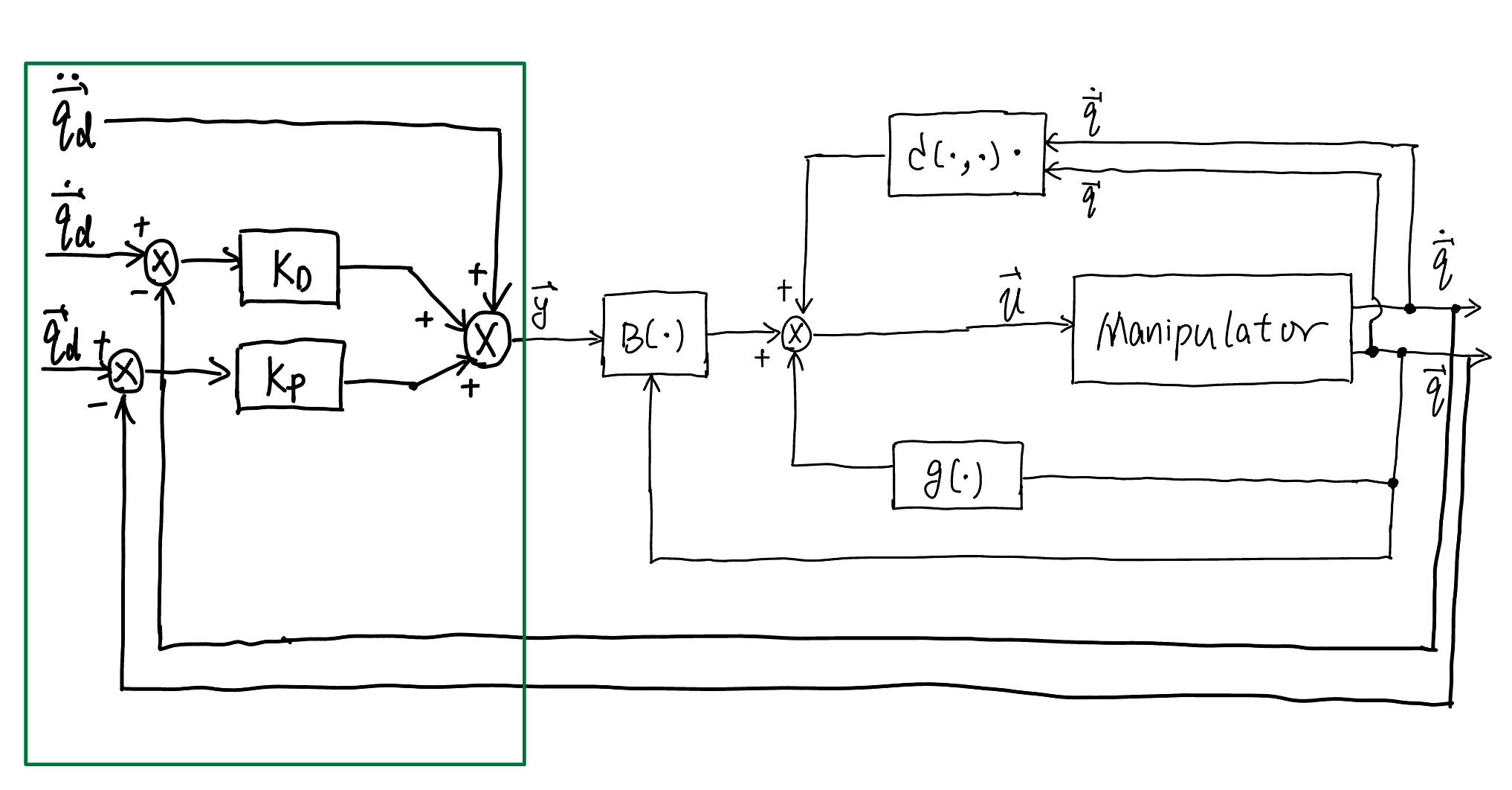
The control block diagram for inverse dynamics control is shown below

../_images/inverse_dynamics_control2.jpeg — Fig. 68 Control diagram of joint space inverse dynamics control#

Controller 3: Impedance Control#

Impedance control specifies a desired dynamic relationship between the joint tracking error and the applied torque so that the robot behaves like a virtual mass-damper-spring system in joint space. In joint coordinates, a common impedance law is

\[\boldsymbol{M}_d\ddot{\tilde{\boldsymbol{e}}}+\boldsymbol{D}_d\dot{\tilde{\boldsymbol{e}}}+\boldsymbol{K}_d\tilde{\boldsymbol{e}}=\boldsymbol{\tau}_{cmd},\]

where

\(\tilde{\boldsymbol{e}}=\boldsymbol{q}-\boldsymbol{q}_d\) is the tracking error (note sign convention),
\(\boldsymbol{M}_d,\boldsymbol{D}_d,\boldsymbol{K}_d\) are the (positive definite) desired inertia, damping and stiffness matrices in joint space,
\(\boldsymbol{\tau}_{cmd}\) is the commanded joint torque that enforces the impedance.

One practical controller that implements joint-space impedance while compensating robot dynamics is

Joint impedance control

The controller for joint impedance control follows:

\[\boldsymbol{\tau}=\boldsymbol{B}(\boldsymbol{q})\boldsymbol{M}_d^{-1}\big(\boldsymbol{K}_d(\boldsymbol{q}_d-\boldsymbol{q})-\boldsymbol{D}_d\dot{\boldsymbol{q}}\big)+\boldsymbol{C}(\boldsymbol{q},\dot{\boldsymbol{q}})\dot{\boldsymbol{q}}+\boldsymbol{g}(\boldsymbol{q}).\]

with \(\boldsymbol{M}_d,\boldsymbol{D}_d,\boldsymbol{K}_d\) are (positive definite) desired inertia, damping and stiffness matrices in joint space.

This controller uses model compensation (the \(\boldsymbol{B},\boldsymbol{C},\boldsymbol{g}\) terms) so that the closed-loop joint dynamics approximate

\[\boldsymbol{M}_d(\ddot{\boldsymbol{q}}-\ddot{\boldsymbol{q}}_d)+\boldsymbol{D}_d(\dot{\boldsymbol{q}}-\dot{\boldsymbol{q}}_d)+\boldsymbol{K}_d(\boldsymbol{q}-\boldsymbol{q}_d)=\boldsymbol{0}.\]

Remarks and design notes:

Choosing \(\boldsymbol{M}_d\) small makes the system more responsive (low apparent inertia); larger \(\boldsymbol{K}_d\) increases stiffness around the desired pose.
Diagonal \(\boldsymbol{M}_d,\boldsymbol{D}_d,\boldsymbol{K}_d\) are common and simplify tuning: pick each joint’s stiffness and damping independently.
If the robot model is uncertain, reduce reliance on full model compensation and add robust terms (e.g., higher damping) or use adaptive/robust control techniques.

Simple discrete-time implementation (control loop at rate \(1/\Delta t\)):

# assume numpy imported as np, and functions get_q(), get_qdot(), send_torque(tau)
M_d = np.diag([0.5]*n)    # desired inertia (example)
D_d = np.diag([5.0]*n)    # desired damping
K_d = np.diag([50.0]*n)   # desired stiffness

def impedance_step(q_d, q_d_dot, q, q_dot):
    e = q - q_d
    v = q_dot - q_d_dot
    # feedforward term (can include desired accel if available)
    tau = B(q) @ np.linalg.solve(M_d, (K_d @ (-e) - D_d @ v)) + C(q, q_dot) @ q_dot + g(q)
    return tau

# in real loop:
# q, q_dot = read_sensors()
# tau_cmd = impedance_step(q_d, q_d_dot, q, q_dot)
# send_torque(tau_cmd)

Include this section as a basis for experiments in class: students can vary \(\boldsymbol{K}_d\) and \(\boldsymbol{D}_d\) to observe compliant vs stiff behavior in simulation or on hardware.

Joint Space Control

Contents

Joint Space Control#

Overview of Robot Control#

Joint Space Control#

Controller 1: PD Control with Gravity Compensation#

Controller 2: Inverse Dynamics Control#

Controller 3: Impedance Control#