Centralized Joint Control

In the previous sections, we have discussed the design of independent (decentralized) joint controllers for each joint. Each joint is viewed as a single input and single-output system, and the coupling effects between the joints considered as disturbances. However, this has the limitation: when the coupling effect is not ignorable, the decentralized performance may be bad. In this case, it would be desirable to design controller that explicitly take into considertaion the coupling effect and compensate for it! This leads to centralized control method in this chapter.

In the following control design for a \(n\)-joint robot arm, we consider a robot arm without external end-effector forces and joint friction. The equation of motion of the robot arm is

(72)\[ \boldsymbol{B}(\boldsymbol{q}) \ddot{\boldsymbol{q}}+\boldsymbol{C}(\boldsymbol{q}, \dot{\boldsymbol{q}}) \dot{\boldsymbol{q}}+\boldsymbol{g}(\boldsymbol{q})=\boldsymbol{\tau}.\]

The controller we want to design is

(73)\[ \boldsymbol{\tau}=\boldsymbol{u}=\textbf{Controller}(\boldsymbol{q}, \boldsymbol{\dot{q}}, \boldsymbol{q}_d, \boldsymbol{\dot{q}}_d)\]

i.e., the controller takes as input the robot’s current joint position \(\boldsymbol{q}\), joint velocity \(\boldsymbol{\dot{q}}\), desired joint position \(\boldsymbol{q}_d\), and desired joint velocity \(\boldsymbol{\dot{q}}_d\), and outputs the joint torque \(\boldsymbol{u}\).

Thus, motion of equation of the robot arm with the controller is

(78)\[ \boldsymbol{B}(\boldsymbol{q}) \ddot{\boldsymbol{q}}+\boldsymbol{C}(\boldsymbol{q}, \dot{\boldsymbol{q}}) \dot{\boldsymbol{q}}+\boldsymbol{g}(\boldsymbol{q})=\textbf{Controller}(\boldsymbol{q}, \boldsymbol{\dot{q}}, \boldsymbol{q}_d, \boldsymbol{\dot{q}}_d)\]

PD Control with Gravity Compensation

Given a stationary desired joint position \(\boldsymbol{q}_{d}\) (here \(\boldsymbol{\dot q}_{d}=\boldsymbol{0}\)), we want to design a controller (73), such that given any initial robot configuration, say \(\boldsymbol{q}_0\), the controlled robot arm (78) will eventually reach \(\boldsymbol{q}_{d}\). If we define the joint error as

\[{\boldsymbol{e}}=\boldsymbol{q}_{d}-\boldsymbol{q}\]

we want

\[\boldsymbol{e}(t)\rightarrow \boldsymbol{0}\quad \text{as}\quad t\rightarrow \infty.\]

Below, we will design the controller (73) based on the Lyapunov method (see background of Lyapunov method in Numerical Inverse Kinematics).

First, we take the vector \(\begin{bmatrix}\boldsymbol{e}\\ \boldsymbol{\dot{q}}\end{bmatrix}\) as the system state vector. Choose the following positive quadratic form as Lyapunov function:

\[V(\dot{\boldsymbol{q}}, {\boldsymbol{e}})=\frac{1}{2} \dot{\boldsymbol{q}}^{T} \boldsymbol{B}(\boldsymbol{q}) \dot{\boldsymbol{q}}+\frac{1}{2} {\boldsymbol{e}}^{T} \boldsymbol{K}_{P} {\boldsymbol{e}} \quad >0 \quad \forall \dot{\boldsymbol{q}}, {\boldsymbol{e}} \neq \mathbf{0}\]

where \(\boldsymbol{K}_{P}\) is an \((n \times n)\) symmetric positive definite matrix. Differentiating \(V(\dot{\boldsymbol{q}}, {\boldsymbol{e}})\) with respect to time, by recalling that \(\boldsymbol{q}_{d}\) is constant (\(\boldsymbol{\dot q}_{d}=\boldsymbol{0}\)), yields

(75)\[\dot{V}=\dot{\boldsymbol{q}}^{T} \boldsymbol{B}(\boldsymbol{q}) \ddot{\boldsymbol{q}}+\frac{1}{2} \dot{\boldsymbol{q}}^{T} \dot{\boldsymbol{B}}(\boldsymbol{q}) \dot{\boldsymbol{q}}-\dot{\boldsymbol{q}}^{T} \boldsymbol{K}_{P} {\boldsymbol{e}}\]

From (72), we can solve for \(\boldsymbol{B} \ddot{\boldsymbol{q}}\) and substituting it to (75) gives

(76)\[\label{equ.lypuanovdot} \dot{V}=\frac{1}{2} \underbrace{\dot{\boldsymbol{q}}^{T}(\dot{\boldsymbol{B}}(\boldsymbol{q})-2 \boldsymbol{C}(\boldsymbol{q}, \dot{\boldsymbol{q}})) \dot{\boldsymbol{q}}}_{0}+\dot{\boldsymbol{q}}^{T}\left(\boldsymbol{u}-\boldsymbol{g}(\boldsymbol{q})-\boldsymbol{K}_{P} {\boldsymbol{e}}\right)\]

The first term on the right-hand side is zero since the matrix \(\dot{\boldsymbol{B}}-2 \boldsymbol{C}\) is a skew-symmetric matrix (see in the property of dynamics in Dynamics). For the second term to be negative, we can set the controller (73) as

(77)\[ \boldsymbol{u}=\underbrace{\boldsymbol{g}(\boldsymbol{q})}_{\text{gravitational compensation}}+\underbrace{\boldsymbol{K}_{P} \boldsymbol{e}}_{\text{proportional control}}\quad\underbrace{-\boldsymbol{K}_{D} \dot{\boldsymbol{q}}}_{\text{derivative control}}\]

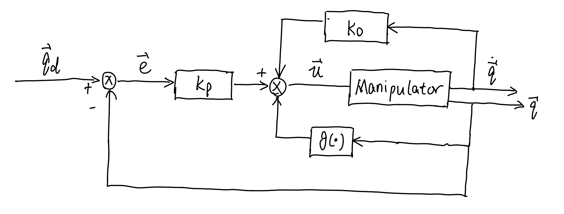
with \(\boldsymbol{K}_{D}\) positive definite matrix. The above controller (77) includes a gravitational compensation term and linear proportional-derivative (PD) control term.

Fig. 80 Control diagram of PD control with gravity compensation

With the above controller (77), the time derivative of the Lyapunov function in (76) becomes

\[\dot{V}=-\boldsymbol{\dot{q}}^T\boldsymbol{K}_D\boldsymbol{\dot{q}} \quad <0 \quad \forall \dot{\boldsymbol{q}} \neq \mathbf{0}\]

and thus, \(V\) decreases long as \(\dot{\boldsymbol{q}} \neq \mathbf{0}\) for all system trajectories. Thus, the robot arm will reach an equilibrium configuration, with condition \(\dot{V}= 0\) and \(\dot{\boldsymbol{q}}=\mathbf{0}\).

To find the equilibrium configuration, we look at the robot dynamics under control (by plug the controller (77) back into (78))

(78)\[\boldsymbol{B}(\boldsymbol{q}) \ddot{\boldsymbol{q}}+\boldsymbol{C}(\boldsymbol{q}, \dot{\boldsymbol{q}}) \dot{\boldsymbol{q}}+\boldsymbol{g}(\boldsymbol{q})=\boldsymbol{g}(\boldsymbol{q})+\boldsymbol{K}_{P} {\boldsymbol{e}}-\boldsymbol{K}_{D} \dot{\boldsymbol{q}}\]

With \(\dot{\boldsymbol{q}}=\mathbf{0}\), it follows that \(\ddot{\boldsymbol{q}} =\mathbf{0}\), and then from the above dynamics (78), we have

\[\boldsymbol{K}_{P} {\boldsymbol{e}}=\mathbf{0} \quad\rightarrow\quad {\boldsymbol{e}}=\boldsymbol{q}_{d}-\boldsymbol{q} = \mathbf{0}\]

Therefore, the robot arm will eventually reach equilibrium, which is exactly the desired configuration \(\boldsymbol{q}_{d}\). In summary, we have the PD controller with gravity compensation for the robot arm, summarized below.

Summary: PD Control with Gravity Compensation

(79)\[ \boldsymbol{u}=\underbrace{\boldsymbol{g}(\boldsymbol{q})}_{\text{gravitational compensation}}+\underbrace{\boldsymbol{K}_{P} (\boldsymbol{q}_d-\boldsymbol{q})}_{\text{proportional control}}\quad\underbrace{-\boldsymbol{K}_{D} \dot{\boldsymbol{q}}}_{\text{derivative control}}\]

with \(\boldsymbol{K}_{P}\) and \(\boldsymbol{K}_{D}\) are positive definite matrices.

Inverse Dynamics Control

One limitation of the PD Control with Gravity Compensation is that the controller can only follow a stationary desired \(\boldsymbol{q}_d\), but is not good at tracking a fast-changing desired joint: i.e.,

(80)\[ \boldsymbol{q}_d(t),\quad\text{with} \quad \boldsymbol{\dot{q}}_d(t)\neq\boldsymbol{0} \quad \text{and} \quad \boldsymbol{\ddot{q}}_d(t)\neq\boldsymbol{0}\]

Inverse dynamics control is to address the above limitation. The idea of inverse dynamics control is to find a controller (73) that can make the robot arm behave like a mass-spring-damper system.

To do so, we set the controller (73) as the following form:

(81)\[ \boldsymbol{u}=\boldsymbol{B}(\boldsymbol{q}) \boldsymbol{y}+\boldsymbol{C}(\boldsymbol{q}, \dot{\boldsymbol{q}}) \dot{\boldsymbol{q}}+\boldsymbol{g}(\boldsymbol{q})\]

where \(\boldsymbol{y}\) is a new input vector which will be determined later on. Plugging the above controller (81) to the robot arm dynamics (72), the controlled robot arm has the dynamics

\[\boldsymbol{B}(\boldsymbol{q}) \ddot{\boldsymbol{q}}+\boldsymbol{C}(\boldsymbol{q}, \dot{\boldsymbol{q}}) \dot{\boldsymbol{q}}+\boldsymbol{g}(\boldsymbol{q})=\boldsymbol{B}(\boldsymbol{q}) \boldsymbol{y}+\boldsymbol{C}(\boldsymbol{q}, \dot{\boldsymbol{q}}) \dot{\boldsymbol{q}}+\boldsymbol{g}(\boldsymbol{q})\]

which is simplified to

(82)\[ \boldsymbol{\ddot{q}}=\boldsymbol{y}\]

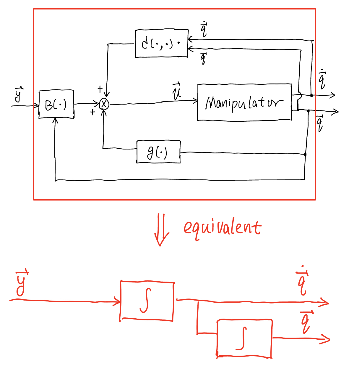
Again, we will discuss how to set this new control input \(\boldsymbol{y}\) later, but (82) shows that the controller (81) leads to a linear relationship between the input signal \(\boldsymbol{y}\) and the robot arm’s joint acceleration \(\ddot{\boldsymbol{q}}\). The following diagram exactly shown this

Fig. 81 Exact linearization performed by inverse dynamics control

How to choose the new input \(\boldsymbol{y}\) in the controller (81)?

For the particular form of controller (81), we choose the new input \(\boldsymbol{y}\) as

(83)\[ \boldsymbol{y}=\ddot{\boldsymbol{{q}}}_d+\boldsymbol{K}_{P} ({\boldsymbol{q}}_{d}-\boldsymbol{q})+\boldsymbol{K}_{D} (\dot{\boldsymbol{q}}_{d}-\dot{\boldsymbol{q}})\]

Here, \(\boldsymbol{K}_{P}\) and \(\boldsymbol{K}_{D}\) are positive definite matrices.

Plugging the above (83) into (82) leads to

(84)\[ (\ddot{\boldsymbol{{q}}}_d-\ddot{\boldsymbol{q}})+\boldsymbol{K}_{P} ({\boldsymbol{q}}_{d}-\boldsymbol{q})+\boldsymbol{K}_{D} (\dot{\boldsymbol{q}}_{d}-\dot{\boldsymbol{q}})=\boldsymbol{0}\]

Again, if we define the error \(\boldsymbol{e}={\boldsymbol{q}}_{d}-{\boldsymbol{q}}\), the above (85) becomes

(85)\[ \ddot{\boldsymbol{e}}+\boldsymbol{K}_{P} \dot{\boldsymbol{e}}+\boldsymbol{K}_{D} {\boldsymbol{e}}=\boldsymbol{0}\]

which is the error dynamics. This is a standard second-order error system, where its convergence depends on the value of \(\boldsymbol{K}_P\) and \(\boldsymbol{K}_D\).

Usually, we usually choose

(86)\[ \boldsymbol{K}_{P}=\operatorname{diag}\left\{\omega_{1}^{2}, \ldots, \omega_{n}^{2}\right\} \quad \boldsymbol{K}_{D}=\operatorname{diag}\left\{2 \zeta_{1} \omega_{1}, \ldots, 2 \zeta_{n} \omega_{n}\right\}\]

Then, the controlled robot arm can be viewed as having \(n\) decoupled (liner) second-order (mass-spring-damper) subsystems. Here, \(\zeta_i\) is the damping ratio and \(\omega_{i}\) the natural frequency for joint \(i\). For each joint \(i\), the error dynamics is

\[ \ddot{{e}}+ 2 \zeta_{i} \omega_{i} \dot{{e}}+ \omega_{i}^{2} {{e}}={0}\]

Please see my Minimal notes on control basics or below for how the values of the damping ratio \(\zeta_i\) and natural frequency \(\omega_{i}\) affect the error response \(\boldsymbol{e}(t)\) in time domain.

Second-order linear system transient response

Given a characteristics equation of a second-order linear system as follows:

\[ s^2+ 2 \zeta \omega_n s+ \omega_n^{2} ={0} \]

with \(\zeta\) called damping ratio and \(\omega_n\) called natural frequency. Both parameters will affect the response of the system in time domain. We have the following empirical equations:

• Settling Time: \(T_s=\frac{4}{\zeta \omega_n}\)

• Peak Time: \(T_p=\frac{\pi}{\omega_n\sqrt{1-\zeta^2}}\)

• Relation between the percent overshoot (\(\%OS\)) and damping ratio \(\zeta\): \(\zeta=\frac{-\ln(\%OS/100)}{\sqrt{\pi^2+\ln^2(\%OS/100)} }\)

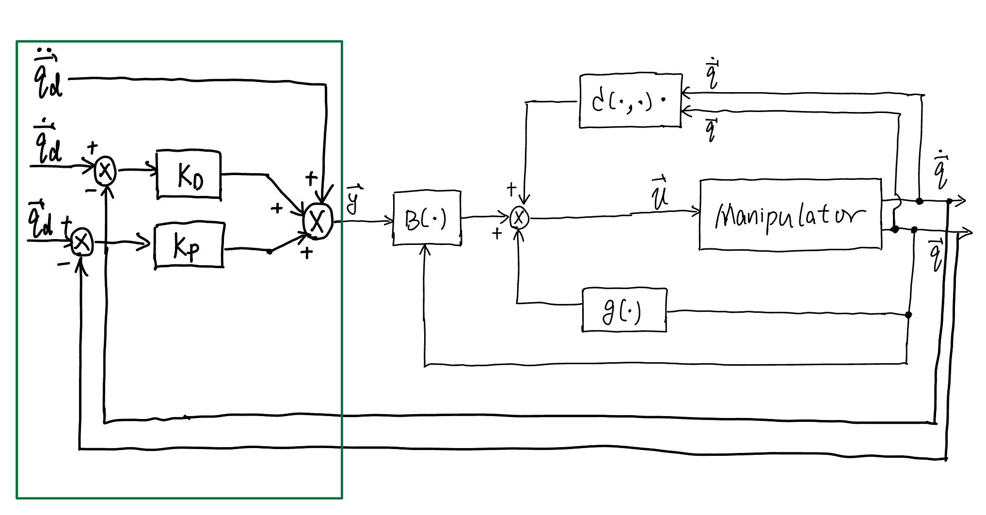
The control block diagram for inverse dynamics control is shown below

Fig. 82 Control diagram of joint space inverse dynamics control

In sum, we recapitulate the joint space inverse dynamics control below

Joint space inverse dynamics control

\[ \boldsymbol{u}=\boldsymbol{B}(\boldsymbol{q}) \boldsymbol{y}+\boldsymbol{C}(\boldsymbol{q}, \dot{\boldsymbol{q}}) \dot{\boldsymbol{q}}+\boldsymbol{g}(\boldsymbol{q})\]

with

\[ \boldsymbol{y}=\ddot{\boldsymbol{{q}}}_d+\boldsymbol{K}_{P} ({\boldsymbol{q}}_{d}-\boldsymbol{q})+\boldsymbol{K}_{D} (\dot{\boldsymbol{q}}_{d}-\dot{\boldsymbol{q}})\]

Here,

\[ \boldsymbol{K}_{P}=\operatorname{diag}\left\{\omega_{1}^{2}, \ldots, \omega_{n}^{2}\right\} \quad \boldsymbol{K}_{D}=\operatorname{diag}\left\{2 \zeta_{1} \omega_{1}, \ldots, 2 \zeta_{n} \omega_{n}\right\}\]

with \(\zeta_i\) the damping ratio and \(\omega_{i}\) the natural frequency for joint \(i\).