Operational Space Control (OSC)

The goal of operational space control (OSC) is to control the robot to track the desired end-effector pose \(\boldsymbol{x}_d\) and velocity \(\boldsymbol{\dot{x}}_d\) given in the operational space.

In the following control design, we consider a a \(n\)-joint robot arm without external end-effector forces and any joint friction. The equation of motion of the robot arm is

(87)\[ \boldsymbol{B}(\boldsymbol{q}) \ddot{\boldsymbol{q}}+\boldsymbol{C}(\boldsymbol{q}, \dot{\boldsymbol{q}}) \dot{\boldsymbol{q}}+\boldsymbol{g}(\boldsymbol{q})=\boldsymbol{u}\]

The controller we want to design is in the general form of

(88)\[ \boldsymbol{u}=\textbf{Controller}(\boldsymbol{q}, \boldsymbol{\dot{q}}, \boldsymbol{x}_d, \boldsymbol{\dot{x}}_d)\]

i.e., the controller takes as input the robot arm’s current joint position \(\boldsymbol{q}\), current joint velocity \(\boldsymbol{\dot{q}}\), the desired end-effector pose \(\boldsymbol{x}_d\), and desired end-effector velocity \(\boldsymbol{\dot{x}}_d\), and outputs the joint torque \(\boldsymbol{u}\).

Thus, the controlled robot arm with the controller has the equation of motion:

(89)\[ \boldsymbol{B}(\boldsymbol{q}) \ddot{\boldsymbol{q}}+\boldsymbol{C}(\boldsymbol{q}, \dot{\boldsymbol{q}}) \dot{\boldsymbol{q}}+\boldsymbol{g}(\boldsymbol{q})=\textbf{Controller}(\boldsymbol{q}, \boldsymbol{\dot{q}}, \boldsymbol{x}_d, \boldsymbol{\dot{x}}_d)\]

In the following, we define the end-effector pose error:

(90)\[ \boldsymbol{e}=\boldsymbol{x}_{d}-\boldsymbol{x} \]

and end-effector velocity error:

(91)\[ \boldsymbol{\dot e}=\boldsymbol{\dot x}_{d}-\boldsymbol{\dot x}=\boldsymbol{\dot x}_{d}-\boldsymbol J (\boldsymbol{q})\boldsymbol{\dot q} \]

with with \(\boldsymbol{x}\) the current/actual robot end-effector pose, and \(\boldsymbol{x}\) the current/actual robot end-effector pose.

OSC PD Control with Gravity Compensation

Given a stationary end-effector pose \(\boldsymbol{x}_{d}\) (i.e., \(\boldsymbol{\dot x}_{ d}=\boldsymbol{0}\)), we want to design a controller (88) such that from any initial robot configuration \(\boldsymbol{q}_0\), the controlled robot arm (89) will eventually reach \(\boldsymbol{x}_{d}\). That means

\[\boldsymbol{e}(t)\rightarrow \boldsymbol{0}\quad \text{as}\quad t\rightarrow \infty\]

Below, we will design the controller (88) based on the Lyapunov method (see background of Lyapunov method in Numerical Inverse Kinematics).

First, we take the vector \(\begin{bmatrix}\boldsymbol{e}\\ \boldsymbol{\dot{q}}\end{bmatrix}\) as the control system state. Choose the following positive definite quadratic form as Lyapunov function:

(92)\[V(\dot{\boldsymbol{q}}, {\boldsymbol{e}})=\frac{1}{2} \dot{\boldsymbol{q}}^{T} \boldsymbol{B}(\boldsymbol{q}) \dot{\boldsymbol{q}}+\frac{1}{2} {\boldsymbol{e}}^{T} \boldsymbol{K}_{P} {\boldsymbol{e}}>0 \quad \forall \dot{\boldsymbol{q}}, {\boldsymbol{e}} \neq \mathbf{0}\]

with \(\boldsymbol{K}_{P}\) a positive definite matrix. Then,

\[\dot{V}=\dot{\boldsymbol{q}}^{T} \boldsymbol{B}(\boldsymbol{q}) \ddot{\boldsymbol{q}}+\frac{1}{2} \dot{\boldsymbol{q}}^{T} \dot{\boldsymbol{B}}(\boldsymbol{q}) \dot{\boldsymbol{q}}+\dot{\boldsymbol{e}}^{T} \boldsymbol{K}_{P} {\boldsymbol{e}}\]

Since \(\dot{\boldsymbol{x}}_{d}=\mathbf{0}\),

\[\dot{{\boldsymbol{e}}}=-\dot{\boldsymbol{x}}=-\boldsymbol{J}(\boldsymbol{q}) \dot{\boldsymbol{q}}\]

and then

(93)\[\dot{V}=\dot{\boldsymbol{q}}^{T} \boldsymbol{B}(\boldsymbol{q}) \ddot{\boldsymbol{q}}+\frac{1}{2} \dot{\boldsymbol{q}}^{T} \dot{\boldsymbol{B}}(\boldsymbol{q}) \dot{\boldsymbol{q}}-\dot{\boldsymbol{q}}^{T} \boldsymbol{J}^{T}(\boldsymbol{q}) \boldsymbol{K}_{P} {\boldsymbol{e}}\]

Similar to the derivation in the previous chapter, we replace \(\boldsymbol{B}\ddot{\boldsymbol{q}}\) in (93) form dynamics (87) and consider the property that \(\dot{\boldsymbol{B}}-2 \boldsymbol{C}\) is a skew-symmetric matrix. Then, (93) becomes

\[\dot{V}=\dot{\boldsymbol{q}}^{T}\left(\boldsymbol{u}-\boldsymbol{g}(\boldsymbol{q})-\boldsymbol{J}_{A}^{T}(\boldsymbol{q}) \boldsymbol{K}_{P} {\boldsymbol{e}}\right) .\]

For the above \(\dot{V}\) to be negative, we choose the controller

(94)\[\boldsymbol{u}=\boldsymbol{g}(\boldsymbol{q})+\boldsymbol{J}^{T}(\boldsymbol{q}) \boldsymbol{K}_{P} {\boldsymbol{e}}-\boldsymbol{J}^{T}(\boldsymbol{q}) \boldsymbol{K}_{D} \boldsymbol{J}(\boldsymbol{q}) \dot{\boldsymbol{q}}\]

with \(\boldsymbol{K}_{D}\) positive definite, then,

(95)\[\dot{V}=-\dot{\boldsymbol{q}}^{T} \boldsymbol{J}^{T}(\boldsymbol{q}) \boldsymbol{K}_{D} \boldsymbol{J}(\boldsymbol{q}) \dot{\boldsymbol{q}} \quad <0, \quad \forall \quad\boldsymbol{\dot{q}}\quad\text{with} \quad \boldsymbol{J}(\boldsymbol{q})\dot{\boldsymbol{q}} \neq \mathbf{0}\]

which says the Lyapunov function decreases as long as \(\boldsymbol{J}(\boldsymbol{q})\dot{\boldsymbol{q}} \neq \mathbf{0}\). Thus, the system reaches an equilibrium pose, with condition \(\dot{V}= 0\) and \(\boldsymbol{J}(\boldsymbol{q})\dot{\boldsymbol{q}}=\mathbf{0}\).

We consider the non-redundant non-singularity of matrix \(\boldsymbol{J}(\boldsymbol{q})\). Then, the equilibrium condition \(\boldsymbol{J}(\boldsymbol{q})\dot{\boldsymbol{q}}=\mathbf{0}\) means that \(\dot{\boldsymbol{q}}=\mathbf{0}\) and further \(\ddot{\boldsymbol{q}} =\mathbf{0}\). To find the robot equilibrium configuration, we look at the robot arm dynamics with controller

(96)\[\boldsymbol{B}(\boldsymbol{q}) \ddot{\boldsymbol{q}}+\boldsymbol{C}(\boldsymbol{q}, \dot{\boldsymbol{q}}) \dot{\boldsymbol{q}}+\boldsymbol{F} \dot{\boldsymbol{q}}+\boldsymbol{g}(\boldsymbol{q})=\boldsymbol{g}(\boldsymbol{q})+\boldsymbol{J}^{T}(\boldsymbol{q}) \boldsymbol{K}_{P} {\boldsymbol{e}}-\boldsymbol{J}^{T}(\boldsymbol{q}) \boldsymbol{K}_{D} \boldsymbol{J}(\boldsymbol{q}) \dot{\boldsymbol{q}}\]

With the condition \(\dot{\boldsymbol{q}}=\mathbf{0}\), it follows that \(\ddot{\boldsymbol{q}} =\mathbf{0}\), and then the above (96) becomes

(97)\[\boldsymbol{J}^{T}(\boldsymbol{q}) \boldsymbol{K}_{P} {\boldsymbol{e}}=\mathbf{0}\quad \rightarrow\quad {\boldsymbol{e}}=\boldsymbol{x}_{d}-\boldsymbol{x}_{e}=\mathbf{0}\]

This concludes that the controlled robot arm will asymptotically reach \(\boldsymbol{x}_d\). The corresponding control diagram is shown below.

Fig. 83 Block diagram of operational space PD control with gravity compensation

Summary: PD Control with Gravity Compensation

(98)\[ \boldsymbol{u}=\underbrace{\boldsymbol{g}(\boldsymbol{q})}_{\text{gravitational compensation}}+ \underbrace{\boldsymbol{J}^{T}(\boldsymbol{q}) \boldsymbol{K}_{P} {(\boldsymbol{x}_d-\boldsymbol{x})}}_{\text{proportional control}}\quad\underbrace{-\boldsymbol{J}^{T}(\boldsymbol{q})\boldsymbol{K}_{D} \boldsymbol{J}(\boldsymbol{q})\dot{\boldsymbol{q}}}_{\text{derivative control}}\]

with \(\boldsymbol{K}_{P}\) and \(\boldsymbol{K}_{D}\) are positive definite matrices.

OSC Inverse Dynamics Control

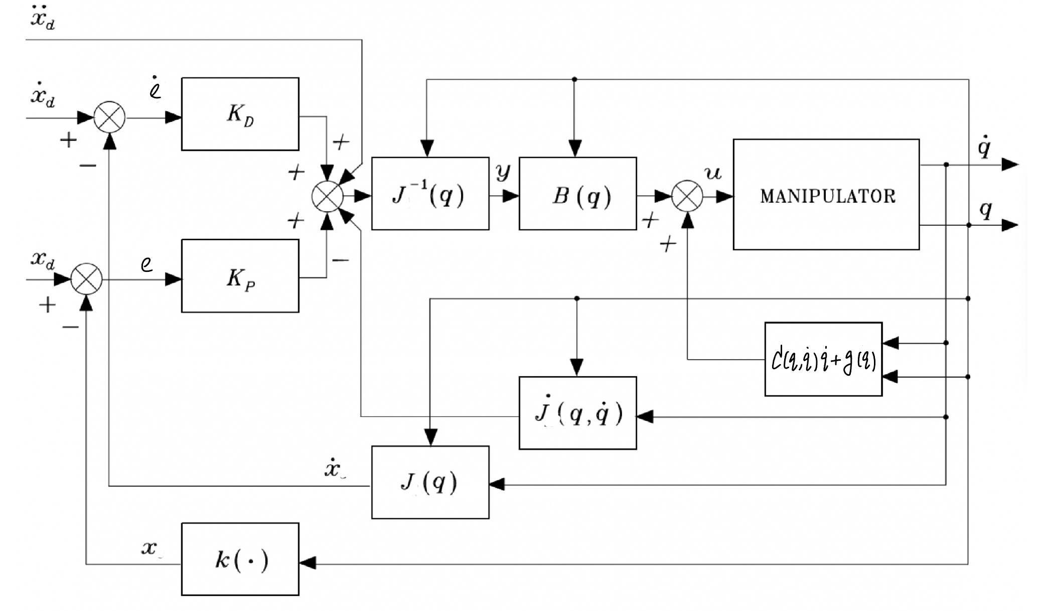
One limitation of the OSC PD Control is that the controller can only follow a stationary desired \(\boldsymbol{x}_d\) , but is not good at tracking a fast-changing desired \(\boldsymbol{x}_d\) (i.e., \(\boldsymbol{\dot x}_d\neq \boldsymbol{0}\)). OSC Inverse Dynamics Control is to address so.

Recall the joint space inverse dynamics control in the previous chapter. If we set the controller as form

(99)\[ \boldsymbol{u}=\boldsymbol{B}(\boldsymbol{q}) \boldsymbol{y}+\boldsymbol{C}(\boldsymbol{q}, \dot{\boldsymbol{q}}) \dot{\boldsymbol{q}}+\boldsymbol{g}(\boldsymbol{q})\]

where \(\boldsymbol{y}\) is a new input vector. The controller directly leads to the controlled robot arm (89) as

(100)\[\boldsymbol{B}(\boldsymbol{q}) \ddot{\boldsymbol{q}}+\boldsymbol{C}(\boldsymbol{q}, \dot{\boldsymbol{q}}) \dot{\boldsymbol{q}}+\boldsymbol{g}(\boldsymbol{q})=\boldsymbol{B}(\boldsymbol{q}) \boldsymbol{y}+\boldsymbol{C}(\boldsymbol{q}, \dot{\boldsymbol{q}}) \dot{\boldsymbol{q}}+\boldsymbol{g}(\boldsymbol{q})\]

further simplified as

(101)\[ \boldsymbol{\ddot{q}}=\boldsymbol{y}\]

Again, we will discuss how to set this new input \(\boldsymbol{y}\) below. The new input \(\boldsymbol{y}\) is designed make the robot arm track a changing \(\boldsymbol{x}_{d}(t)\). To this end, we differentiate the jacobian equation

\[\dot{\boldsymbol{x}}=\boldsymbol{J}(\boldsymbol{q})\dot{\boldsymbol{q}}\]

on both side with respect to time \(t\), leading to

(102)\[ \ddot{\boldsymbol{x}}=\boldsymbol{J}(\boldsymbol{q}) \ddot{\boldsymbol{q}}+\dot{\boldsymbol{J}}(\boldsymbol{q}, \dot{\boldsymbol{q}}) \dot{\boldsymbol{q}}\]

The above (102) suggests the following choice of \(\boldsymbol{y}\):

(103)\[ \boldsymbol{y}=\boldsymbol{J}^{-1}(\boldsymbol{q})\left(\ddot{\boldsymbol{x}}_{d}+\boldsymbol{K}_{D} \dot{{\boldsymbol{e}}}+\boldsymbol{K}_{P} {\boldsymbol{e}}-\dot{\boldsymbol{J}}(\boldsymbol{q}, \dot{\boldsymbol{q}}) \dot{\boldsymbol{q}}\right)\]

with \(\boldsymbol{K}_{P}\) and \(\boldsymbol{K}_{D}\) positive definite matrices. In fact, plugging (103) to (102) leads to the error dynamics

\[\ddot{{\boldsymbol{e}}}+\boldsymbol{K}_{D} \dot{{\boldsymbol{e}}}+\boldsymbol{K}_{P} {\boldsymbol{e}}=\mathbf{0}\]

which describes the operational space error dynamics, with \(\boldsymbol{K}_{P}\) and \(\boldsymbol{K}_{D}\) determining the error convergence rate to zero. Typicaly we choose

\[ \boldsymbol{K}_{P}=\operatorname{diag}\left\{\omega_{1}^{2}, \ldots, \omega_{r}^{2}\right\} \quad \boldsymbol{K}_{D}=\operatorname{diag}\left\{2 \zeta_{1} \omega_{1}, \ldots, 2 \zeta_{r} \omega_{r}\right\}\]

with with \(\zeta_i\) the damping ratio and \(\omega_{i}\) the natural frequency. Then, the end-effector of the controlled robot arm will behave like a linear second-order (mass-spring-damper) system.

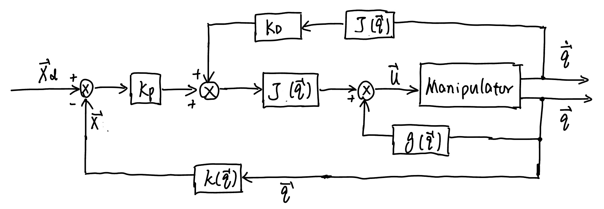
The resulting OCS inverse dynamics control diagram is shown below.

Fig. 84 Block scheme of operational space PD control with gravity compensation

In sum, we recapitulate the operational space inverse dynamics control below

OCS inverse dynamics control

\[ \boldsymbol{u}=\boldsymbol{B}(\boldsymbol{q}) \boldsymbol{y}+\boldsymbol{C}(\boldsymbol{q}, \dot{\boldsymbol{q}}) \dot{\boldsymbol{q}}+\boldsymbol{g}(\boldsymbol{q})\]

with

\[ \boldsymbol{y}=\boldsymbol{J}^{-1}(\boldsymbol{q})\left(\ddot{\boldsymbol{x}}_{d}+\boldsymbol{K}_{D} \dot{{\boldsymbol{e}}}+\boldsymbol{K}_{P} {\boldsymbol{e}}-\dot{\boldsymbol{J}}(\boldsymbol{q}, \dot{\boldsymbol{q}}) \dot{\boldsymbol{q}}\right)\]

Here,

\[ \boldsymbol{K}_{P}=\operatorname{diag}\left\{\omega_{1}^{2}, \ldots, \omega_{r}^{2}\right\} \quad \boldsymbol{K}_{D}=\operatorname{diag}\left\{2 \zeta_{1} \omega_{1}, \ldots, 2 \zeta_{r} \omega_{r}\right\}\]

with with \(\zeta_i\) the damping ratio and \(\omega_{i}\) the natural frequency.